Assignment 3: Tidying & Importing Data

Due by 11:59 PM on Sunday, April 26, 2026

Assignment Details

Assigned: Monday, April 20 (Session 7) Due: Sunday, April 26 at 11:59 PM Submit: Quarto document (.qmd) AND rendered HTML on Canvas

First Quarto assignment!

This is the first assignment submitted as a Quarto document. See the guides: Setting Up an R Project | Using Quarto Documents

Overview

This assignment practices reshaping data with pivot_longer() and pivot_wider(), and importing data from CSV files. You’ll work with psychology-style datasets.

Setup

# Assignment 3: Tidying & Importing Data
# Your Name
# Date

library(tidyverse)

Part 1: Pivoting Wide to Long (30 points)

A researcher collected anxiety scores at three time points. The data is in “wide” format:

anxiety_wide <- tibble(
  participant_id = 1:5,
  condition = c("treatment", "treatment", "control", "control", "treatment"),
  anxiety_t1 = c(45, 52, 48, 55, 42),
  anxiety_t2 = c(38, 45, 47, 54, 35),
  anxiety_t3 = c(32, 40, 46, 52, 30)
)

Task 1.1

Pivot this data to long format so you have columns for:

participant_id
condition
time (values: “t1”, “t2”, “t3”)
anxiety (the score)

Answer

anxiety_long <- anxiety_wide |>
  pivot_longer(
    cols = starts_with("anxiety_"),
    names_to = "time",
    values_to = "anxiety",
    names_prefix = "anxiety_"
  )

anxiety_long

# A tibble: 15 × 4
   participant_id condition time  anxiety
            <int> <chr>     <chr>   <dbl>
 1              1 treatment t1         45
 2              1 treatment t2         38
 3              1 treatment t3         32
 4              2 treatment t1         52
 5              2 treatment t2         45
 6              2 treatment t3         40
 7              3 control   t1         48
 8              3 control   t2         47
 9              3 control   t3         46
10              4 control   t1         55
11              4 control   t2         54
12              4 control   t3         52
13              5 treatment t1         42
14              5 treatment t2         35
15              5 treatment t3         30

names_prefix = "anxiety_" strips the prefix so you get clean labels (t1, t2, t3) instead of anxiety_t1, etc.

Task 1.2

Using your long dataset, calculate the mean anxiety score at each time point, separately for each condition.

Answer

Tip

This builds on Task 1.1 — anxiety_long must exist first.

anxiety_means <- anxiety_long |>
  group_by(condition, time) |>
  summarise(mean_anxiety = mean(anxiety), .groups = "drop")

anxiety_means

# A tibble: 6 × 3
  condition time  mean_anxiety
  <chr>     <chr>        <dbl>
1 control   t1            51.5
2 control   t2            50.5
3 control   t3            49  
4 treatment t1            46.3
5 treatment t2            39.3
6 treatment t3            34

Task 1.3

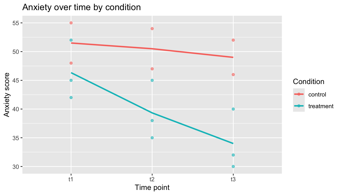
Create a line plot showing anxiety over time, with separate lines for each condition. Add points for the individual observations.

Answer

The cleanest version uses stat_summary() so the line is computed from the data and the individual observations are still visible as points.

ggplot(anxiety_long, aes(x = time, y = anxiety,
                         colour = condition, group = condition)) +
  geom_point(alpha = 0.6) +
  stat_summary(fun = mean, geom = "line", linewidth = 1) +
  labs(
    title = "Anxiety over time by condition",
    x = "Time point",
    y = "Anxiety score",
    colour = "Condition"
  )

Line plot of anxiety scores at three time points (t1, t2, t3), with separate lines for treatment and control conditions and individual participant observations shown as points. Treatment shows a clear decline; control stays roughly flat.

Part 2: Pivoting Long to Wide (25 points)

A survey measured different emotions. The data is in long format:

emotions_long <- tibble(
  participant = rep(1:4, each = 3),
  emotion = rep(c("happy", "sad", "anxious"), 4),
  rating = c(7, 2, 3, 5, 4, 6, 8, 1, 2, 6, 5, 4)
)

Task 2.1

Pivot this to wide format so each emotion is its own column.

Answer

emotions_wide <- emotions_long |>
  pivot_wider(names_from = emotion, values_from = rating)

emotions_wide

# A tibble: 4 × 4
  participant happy   sad anxious
        <int> <dbl> <dbl>   <dbl>
1           1     7     2       3
2           2     5     4       6
3           3     8     1       2
4           4     6     5       4

The column order (happy / sad / anxious) reflects the order the emotions appear in the data. That’s fine.

Task 2.2

Using the wide format, create a new variable that is the sum of all three emotion ratings for each participant.

Answer

Tip

This builds on Task 2.1 — emotions_wide must exist first.

emotions_wide |>
  mutate(total = happy + sad + anxious)

# A tibble: 4 × 5
  participant happy   sad anxious total
        <int> <dbl> <dbl>   <dbl> <dbl>
1           1     7     2       3    12
2           2     5     4       6    15
3           3     8     1       2    11
4           4     6     5       4    15

Part 3: Importing Data (35 points)

Download the provided data files from Canvas and save them in your project’s data/raw/ folder:

survey_data.csv — Survey responses with some messy formatting
demographics.xlsx — Participant demographics in Excel format

Task 3.1

Import survey_data.csv using read_csv(). Note any warnings or issues.

Answer

survey_first <- read_csv("../files/data/survey_data.csv")
glimpse(survey_first)

Rows: 20
Columns: 6
$ participant_id <dbl> 101, 102, 103, 104, 105, 106, 107, 108, 109, 110, 111, …
$ condition      <chr> "treatment", "control", "treatment", "control", "treatm…
$ pre_anxiety    <dbl> 62, 55, 70, 48, 75, 61, 58, 52, 80, 67, 63, 50, 72, 57,…
$ post_anxiety   <chr> "45", "N/A", "52", "50", "58", "N/A", "42", "55", "65",…
$ pre_wellbeing  <dbl> 28, 31, 22, 38, 18, 30, 33, 35, 15, 27, 29, 36, 20, 32,…
$ post_wellbeing <chr> "35", "N/A", "32", "36", "28", "N/A", "40", "34", "25",…

Notice that post_anxiety and post_wellbeing come in as character instead of numeric. That’s because the literal string "N/A" appears in those columns, and read_csv() doesn’t know it’s meant to represent a missing value. We’ll fix that in Task 3.2.

Task 3.2

The CSV has some problems:

Missing values are coded as “N/A” instead of blank
Some columns have wrong types

Re-import the data handling these issues using the appropriate read_csv() arguments (hint: na = and col_types =).

Answer

Setting na = "N/A" is enough on its own — once the strings are treated as missing, the columns parse as numeric automatically.

survey <- read_csv("../files/data/survey_data.csv", na = "N/A")
glimpse(survey)

Rows: 20
Columns: 6
$ participant_id <dbl> 101, 102, 103, 104, 105, 106, 107, 108, 109, 110, 111, …
$ condition      <chr> "treatment", "control", "treatment", "control", "treatm…
$ pre_anxiety    <dbl> 62, 55, 70, 48, 75, 61, 58, 52, 80, 67, 63, 50, 72, 57,…
$ post_anxiety   <dbl> 45, NA, 52, 50, 58, NA, 42, 55, 65, NA, 48, 52, 55, 58,…
$ pre_wellbeing  <dbl> 28, 31, 22, 38, 18, 30, 33, 35, 15, 27, 29, 36, 20, 32,…
$ post_wellbeing <dbl> 35, NA, 32, 36, 28, NA, 40, 34, 25, NA, 37, 34, 30, 32,…

If you want to be explicit about column types, you can add col_types:

read_csv(
  "../files/data/survey_data.csv",
  na = "N/A",
  col_types = cols(
    participant_id  = col_integer(),
    condition       = col_character(),
    pre_anxiety     = col_double(),
    post_anxiety    = col_double(),
    pre_wellbeing   = col_double(),
    post_wellbeing  = col_double()
  )
)

Task 3.3

Import demographics.xlsx using the readxl package. The data is on the second sheet.

library(readxl)
# Your code here

Answer

demographics <- read_excel("../files/data/demographics.xlsx", sheet = 2)
demographics

# A tibble: 18 × 5
   participant_id   age gender year_in_school major            
            <dbl> <dbl> <chr>  <chr>          <chr>            
 1            101    19 F      Freshman       Psychology       
 2            102    22 M      Senior         Neuroscience     
 3            103    20 F      Sophomore      Psychology       
 4            104    21 F      Junior         Sociology        
 5            105    23 M      Senior         Psychology       
 6            106    19 F      Freshman       Biology          
 7            107    22 M      Junior         Psychology       
 8            108    20 F      Sophomore      Cognitive Science
 9            109    21 M      Junior         Neuroscience     
10            110    19 F      Freshman       Psychology       
11            111    24 F      Senior         Sociology        
12            112    22 M      Junior         Psychology       
13            113    20 F      Sophomore      Cognitive Science
14            114    21 M      Junior         Biology          
15            115    19 F      Freshman       Psychology       
16            116    22 M      Senior         Neuroscience     
17            117    20 F      Sophomore      Psychology       
18            118    23 M      Senior         Sociology

You can also reference the sheet by name (sheet = "demographics"), which is more readable. Watch out: sheet 1 is the codebook (5 rows describing each variable), not the demographics data. Make sure you’re pulling sheet 2.

Grading Rubric

Task	Points
1.1: Pivot to long format	10
1.2: Calculate means by time and condition	10
1.3: Create line plot	10
2.1: Pivot to wide format	15
2.2: Create sum of emotion ratings	10
3.1: Import CSV with `read_csv()`	10
3.2: Re-import handling NA values and column types	15
3.3: Import Excel with `readxl`	10
QMD file knits without errors	10
Total	100

Grading scale per task: Full points = correct. Full - 1 = one minor error (typo, small formatting issue). Half credit = one major error. 0 = not attempted or multiple major errors. “QMD file knits” refers to whether the Quarto document renders successfully, not whether individual code produces correct output.

Submission

All pivot operations produce correct output
CSV and Excel files imported successfully
Document renders without errors

Submit your .qmd file and your rendered .html file on Canvas.

PSY 510 (Graduate Students)

Students enrolled in PSY 510 must complete the following extension in addition to all tasks above.

Graduate Extension: Qualtrics API

Most psychology researchers collect data through Qualtrics. Instead of logging in and downloading a CSV by hand, you can pull data directly into R using the qualtRics package — a workflow that scales to repeated data collection and eliminates manual steps that introduce error.

For this extension you’ll pull data from the anonymous start-of-term survey that your classmates completed in Week 1. Because it was collected anonymously, the data are safe to work with directly — no masking needed.

Setup

# install.packages("qualtRics")
library(qualtRics)

Task G.1

Authenticate with the Qualtrics API using your UO API key and data center ID. You’ll find both in Qualtrics under Account Settings → Qualtrics IDs.

qualtrics_api_credentials(
  api_key  = "YOUR_API_KEY",
  base_url = "YOUR_DATACENTER.qualtrics.com"
)

Task G.2

Pull responses from the start-of-term survey using fetch_survey(). The survey ID is posted on Canvas.

survey_id <- "SV_XXXXXXXXXXXXXXX"  # replace with actual ID from Canvas
raw <- fetch_survey(surveyID = survey_id)
glimpse(raw)

Task G.3

The raw API output includes a lot of Qualtrics metadata columns (timing, location, status flags) alongside the actual responses. Select only the columns that correspond to the survey questions and give them informative names.

Task G.4

Compare your cleaned API output to the manually exported CSV version of the same survey (posted on Canvas). Note at least two differences in column names, data types, or structure. What would you need to do to make them match exactly?

Task G.5

Write a short reflection (~half a page) answering: When would you use the API rather than a manual export in your own research? What are the tradeoffs in terms of effort, reliability, and reproducibility?

Submission: Add your code and reflection to your .qmd file under a clearly marked ## Graduate Extension section.