Assignment 1: Getting Started with R

Due by 11:59 PM on Sunday, April 5, 2026

Assignment Details

Assigned: Wednesday, April 1 (Session 2) Due: Sunday, April 5 at 11:59 PM Submit: R script (.R file) on Canvas

New to R?

See the step-by-step guides: Setting Up an R Project | Using R Scripts

Overview

This assignment gets you comfortable with RStudio and introduces you to creating visualizations with ggplot2. You’ll work with the built-in mpg dataset to create your first plots.

Setup

Open RStudio and your psy410 project
Create a new R script: File → New File → R Script
Save it as assignment-01-YOURNAME.R
At the top of your script, add:

# Assignment 1: Getting Started with R
# Your Name
# Date

library(tidyverse)

Tasks

Task 1: Explore the data (10 points)

Use the mpg dataset (loaded automatically with tidyverse).

Use glimpse() to look at the structure of mpg. In a comment, note how many rows and columns there are.
Use ?mpg to read the documentation. In a comment, explain what displ and hwy represent.

Answer

Part a: glimpse() gives you a quick overview of the structure.

glimpse(mpg)

Rows: 234
Columns: 11
$ manufacturer <chr> "audi", "audi", "audi", "audi", "audi", "audi", "audi", "…
$ model        <chr> "a4", "a4", "a4", "a4", "a4", "a4", "a4", "a4 quattro", "…
$ displ        <dbl> 1.8, 1.8, 2.0, 2.0, 2.8, 2.8, 3.1, 1.8, 1.8, 2.0, 2.0, 2.…
$ year         <int> 1999, 1999, 2008, 2008, 1999, 1999, 2008, 1999, 1999, 200…
$ cyl          <int> 4, 4, 4, 4, 6, 6, 6, 4, 4, 4, 4, 6, 6, 6, 6, 6, 6, 8, 8, …
$ trans        <chr> "auto(l5)", "manual(m5)", "manual(m6)", "auto(av)", "auto…
$ drv          <chr> "f", "f", "f", "f", "f", "f", "f", "4", "4", "4", "4", "4…
$ cty          <int> 18, 21, 20, 21, 16, 18, 18, 18, 16, 20, 19, 15, 17, 17, 1…
$ hwy          <int> 29, 29, 31, 30, 26, 26, 27, 26, 25, 28, 27, 25, 25, 25, 2…
$ fl           <chr> "p", "p", "p", "p", "p", "p", "p", "p", "p", "p", "p", "p…
$ class        <chr> "compact", "compact", "compact", "compact", "compact", "c…

# 234 rows, 11 columns

Part b: ?mpg opens the help page in RStudio — run this in your console, it won’t produce output in a document.

?mpg

# displ: engine displacement, in litres — a measure of engine size.
#         Larger values = bigger engine.
# hwy: highway miles per gallon — fuel efficiency on the highway.
#       Larger values = better fuel economy.

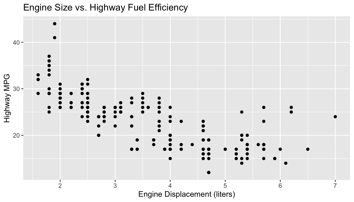
Task 2: Create a basic scatterplot (15 points)

Create a scatterplot showing the relationship between engine displacement (displ) and highway fuel efficiency (hwy).

Your plot should:

Have displacement on the x-axis
Have highway mpg on the y-axis
Include a clear title
Have labeled axes (not just variable names)

Answer

ggplot(mpg, aes(x = displ, y = hwy)) +
  geom_point() +
  labs(
    title = "Engine Size vs. Highway Fuel Efficiency",
    x = "Engine Displacement (liters)",
    y = "Highway MPG"
  )

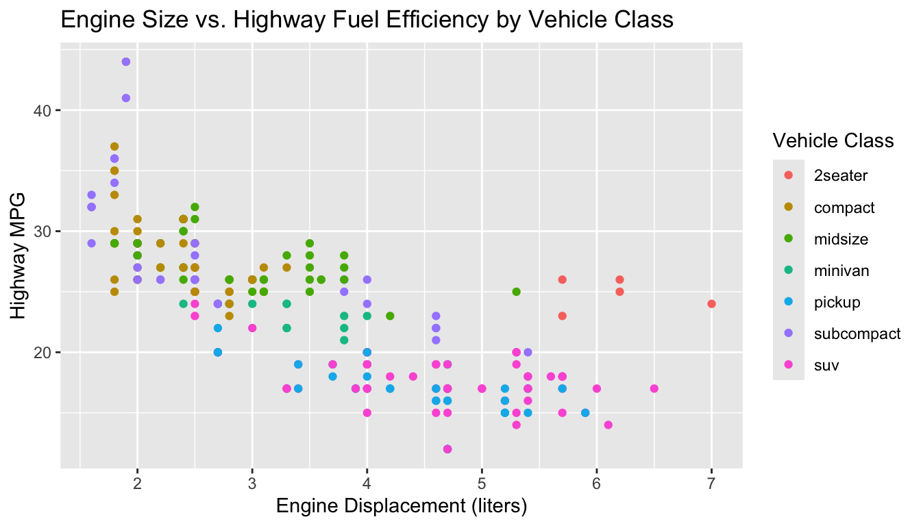
Task 3: Add color (20 points)

Modify your scatterplot to color the points by vehicle class (class).

The legend should appear automatically
Give the legend a clear title (hint: use labs())

Answer

ggplot(mpg, aes(x = displ, y = hwy, color = class)) +
  geom_point() +
  labs(
    title = "Engine Size vs. Highway Fuel Efficiency by Vehicle Class",
    x = "Engine Displacement (liters)",
    y = "Highway MPG",
    color = "Vehicle Class"
  )

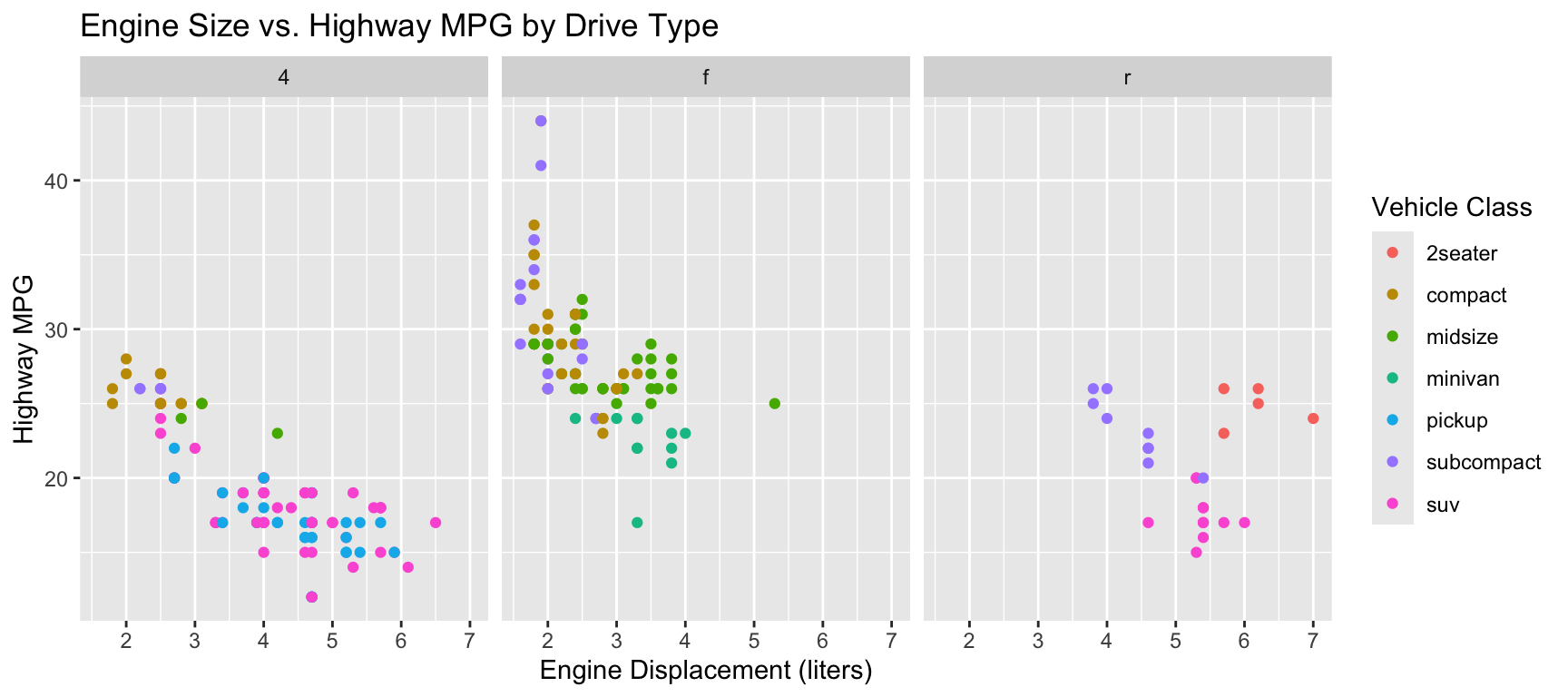
Task 4: Create faceted plots (20 points)

Create the same scatterplot (displacement vs highway mpg, colored by class), but now faceted by drive type (drv).

Use facet_wrap()
Each panel should be clearly labeled

Answer

ggplot(mpg, aes(x = displ, y = hwy, color = class)) +
  geom_point() +
  facet_wrap(~drv) +
  labs(
    title = "Engine Size vs. Highway MPG by Drive Type",
    x = "Engine Displacement (liters)",
    y = "Highway MPG",
    color = "Vehicle Class"
  )

The three panels are 4 (four-wheel drive), f (front-wheel drive), and r (rear-wheel drive). Rear-wheel drive vehicles cluster at high displacement and low mpg — mostly sports cars and trucks.

Task 5: Save your plot (15 points)

Save your final faceted plot as a PNG file.

ggsave("mpg_faceted_plot.png", width = 10, height = 6)

Verify the file was created in your project folder.

Answer

ggsave() saves the most recently created plot. Run this immediately after your ggplot() code.

ggsave("mpg_faceted_plot.png", width = 10, height = 6)

If you want to be explicit about which plot to save, store it in an object first:

my_plot <- ggplot(mpg, aes(x = displ, y = hwy, color = class)) +
  geom_point() +
  facet_wrap(~drv) +
  labs(
    title = "Engine Size vs. Highway MPG by Drive Type",
    x = "Engine Displacement (liters)",
    y = "Highway MPG",
    color = "Vehicle Class"
  )

ggsave("mpg_faceted_plot.png", plot = my_plot, width = 10, height = 6)

Check your Files pane in RStudio — mpg_faceted_plot.png should appear in your project folder.

Task 6: Reflection (10 points)

At the bottom of your script, answer these questions in comments:

# Reflection Questions:
# 1. What relationship do you observe between engine size and fuel efficiency?
# 2. Do all vehicle classes follow the same pattern?
# 3. What was the most challenging part of this assignment?

Sample Answers

Reflection questions don’t have a single right answer, but here’s what a strong response looks like:

# 1. What relationship do you observe between engine size and fuel efficiency?
# There is a clear negative relationship: as engine displacement increases,
# highway fuel efficiency decreases. Larger engines tend to get fewer miles
# per gallon.

# 2. Do all vehicle classes follow the same pattern?
# Mostly yes, but there are differences by class. SUVs and pickups cluster
# in the high-displacement, low-mpg region. Compact and midsize cars cluster
# in the low-displacement, high-mpg region. When faceted by drive type,
# rear-wheel drive vehicles are almost entirely large-engine, low-efficiency
# vehicles (sports cars and pickups). Front-wheel drive vehicles span a wider
# range of engine sizes but have better fuel economy overall.

# 3. What was the most challenging part of this assignment?
# (Individual answer — common responses: file paths for ggsave, figuring out
# where the PNG was saved, understanding the difference between color inside
# vs. outside aes().)

Submission Checklist

Before submitting, make sure:

Your script runs without errors from start to finish
All tasks are completed with code and comments
Your PNG file was created successfully
Your name is at the top of the script

Submit your .R file on Canvas.

Grading Rubric

Task	Points
Task 1: Data exploration	10
Task 2: Basic scatterplot	15
Task 3: Color mapping	20
Task 4: Faceting	20
Task 5: Saving plot	15
Task 6: Reflection	10
Code runs without errors	10
Total	100