Joins

PSY 410: Data Science for Psychology

Dr. Sara Weston

2026-05-20

Why join data?

Three files, one question

Your participant took a survey on Monday and did a cognitive task on Tuesday. The survey data is in one CSV. The task data is in another. Their demographics are in a third.

You want to ask: “Did anxious participants respond more slowly?”

You can’t answer that from any single file. You need joins — the tool that connects separate tables through a shared key.

Open by asking students if they have ever tried to combine two spreadsheets by hand — copying and pasting columns, sorting to line things up. That pain point is the motivation for today. Spend ~3 minutes here. This example (survey + task + demographics) maps directly onto what many of them will face in their final projects.

Two tables, one question

Let’s start simple with just two of the three files — participants and the survey.

# Participant information
participants <- tibble(
  participant_id = 1:4,
  age = c(22, 25, 19, 31),
  condition = c("Control", "Treatment", "Treatment", "Control")
)

# Survey responses (collected separately)
survey <- tibble(
  participant_id = c(1, 2, 3, 5),  # Note: 4 is missing, 5 is extra
  depression = c(12, 18, 10, 25),
  anxiety = c(15, 20, 12, 30)
)

The two tables

Participants:

participants

# A tibble: 4 × 3
  participant_id   age condition
           <int> <dbl> <chr>    
1              1    22 Control  
2              2    25 Treatment
3              3    19 Treatment
4              4    31 Control  

Survey:

survey

# A tibble: 4 × 3
  participant_id depression anxiety
           <dbl>      <dbl>   <dbl>
1              1         12      15
2              2         18      20
3              3         10      12
4              5         25      30

How do we combine these based on participant_id?

Point out the deliberate mismatch: participant 4 is in the left table but not the right, and participant 5 is in the right but not the left. Ask students to predict what should happen to those rows. This asymmetry is the whole reason different join types exist, and it will recur throughout the deck.

Keys

What are keys?

Keys are variables that uniquely identify observations and connect tables.

Primary key: Uniquely identifies each observation in a table

• participant_id in the participants table
• Each participant appears only once

Foreign key: References the primary key of another table

• participant_id in the survey table
• Links back to the participants table

Students sometimes confuse keys with row numbers. Emphasize that a key is a meaningful identifier that lives in the data itself, not the row index. A useful analogy: your student ID number follows you across the registrar, financial aid, and library systems — it is the key that links your records across those separate databases.

Checking for unique keys

Before joining, verify that your key truly identifies each row:

# Check if participant_id is unique
participants |>
  count(participant_id) |>
  filter(n > 1)

# A tibble: 0 × 2
# ℹ 2 variables: participant_id <int>, n <int>

Empty result = good! Each participant appears only once.

When keys aren’t unique

Sometimes keys aren’t unique (e.g., longitudinal data):

longitudinal <- tibble(
  participant_id = c(1, 1, 2, 2, 3, 3),
  timepoint = c(1, 2, 1, 2, 1, 2),
  depression = c(20, 15, 18, 12, 25, 22)
)

Here, the combination of participant_id + timepoint is the key:

longitudinal |>
  count(participant_id, timepoint) |>
  filter(n > 1)

# A tibble: 0 × 3
# ℹ 3 variables: participant_id <dbl>, timepoint <dbl>, n <int>

This is a common point of confusion. Students think “participant_id is always the key,” but in repeated-measures data it is not unique on its own. Ask them: “If you have 3 participants measured at 2 timepoints, how many rows do you have?” This sets up the compound key idea naturally. The count-and-filter pattern for checking uniqueness is worth having them type out — they will use it often.

Mutating joins

The join family

Mutating joins add columns from one table to another:

Function	Keeps rows from…
left_join()	Left table (all rows)
right_join()	Right table (all rows)
inner_join()	Both tables (only matches)
full_join()	Both tables (all rows)

Pause here and explain why they are called “mutating” joins — like mutate(), they add new columns. The table is a reference slide; don’t belabor it. Tell students you will walk through each type one at a time with the same example so they can see exactly how the output differs. Spend ~1 minute on this overview before moving on.

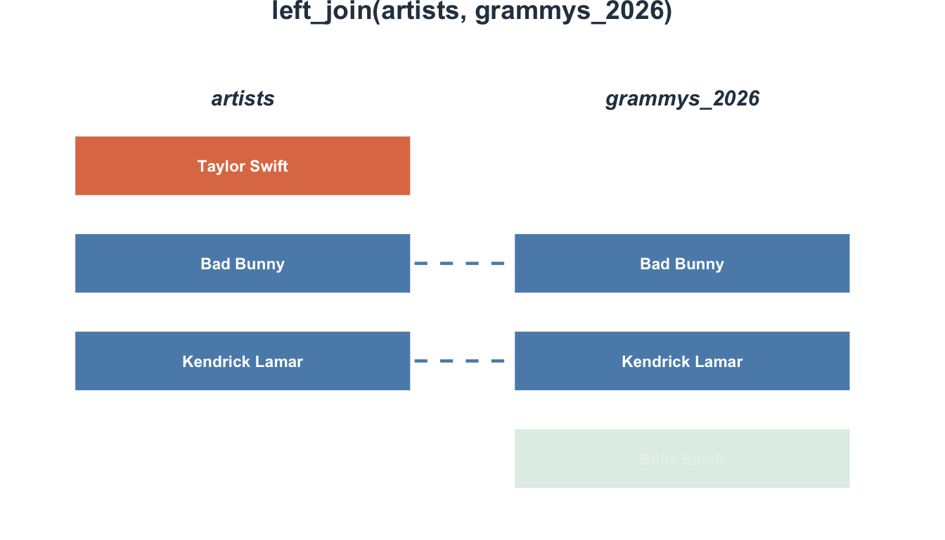
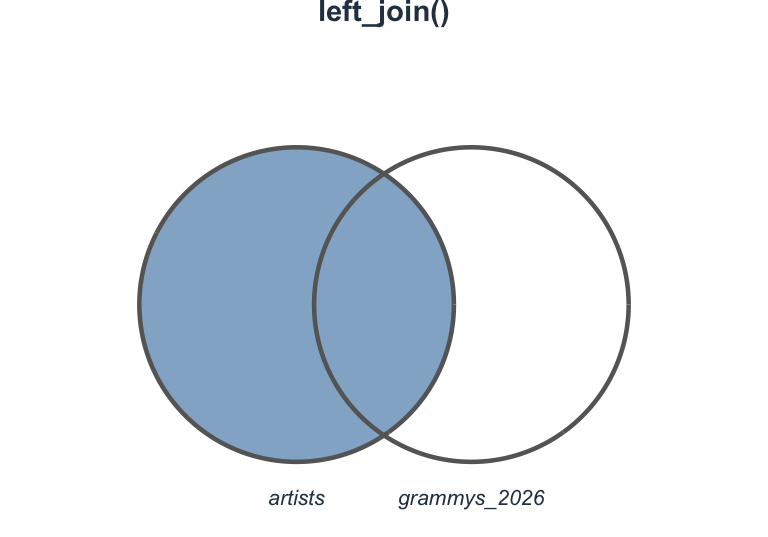
left_join(): Most common

Keep all rows from the left table, add matching data from the right:

participants |>
  left_join(survey, by = "participant_id")

# A tibble: 4 × 5
  participant_id   age condition depression anxiety
           <dbl> <dbl> <chr>          <dbl>   <dbl>
1              1    22 Control           12      15
2              2    25 Treatment         18      20
3              3    19 Treatment         10      12
4              4    31 Control           NA      NA

• Participant 4 has no survey data → NA
• Participant 5 from survey isn’t in participants → excluded

This is the most important slide in the first half of the deck. Walk through the output row by row. Ask: “Why does participant 4 have NA for depression and anxiety?” and “Where did participant 5 go?” Students often ask whether the left table is the one before the pipe or the one inside left_join() — clarify that the piped-in table is always the left table. Spend ~3 minutes here.

Visualizing left_join()

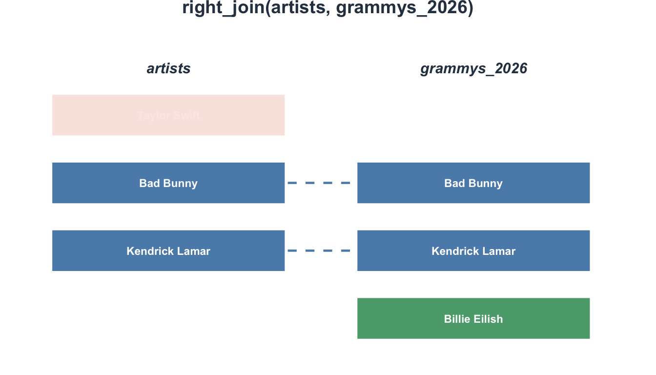
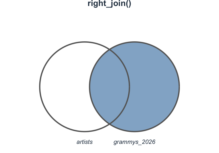
right_join(): The mirror

Keep all rows from the right table:

participants |>
  right_join(survey, by = "participant_id")

# A tibble: 4 × 5
  participant_id   age condition depression anxiety
           <dbl> <dbl> <chr>          <dbl>   <dbl>
1              1    22 Control           12      15
2              2    25 Treatment         18      20
3              3    19 Treatment         10      12
4              5    NA <NA>              25      30

Now participant 5 is included (with NA for age/condition), but participant 4 is excluded.

Visualizing right_join()

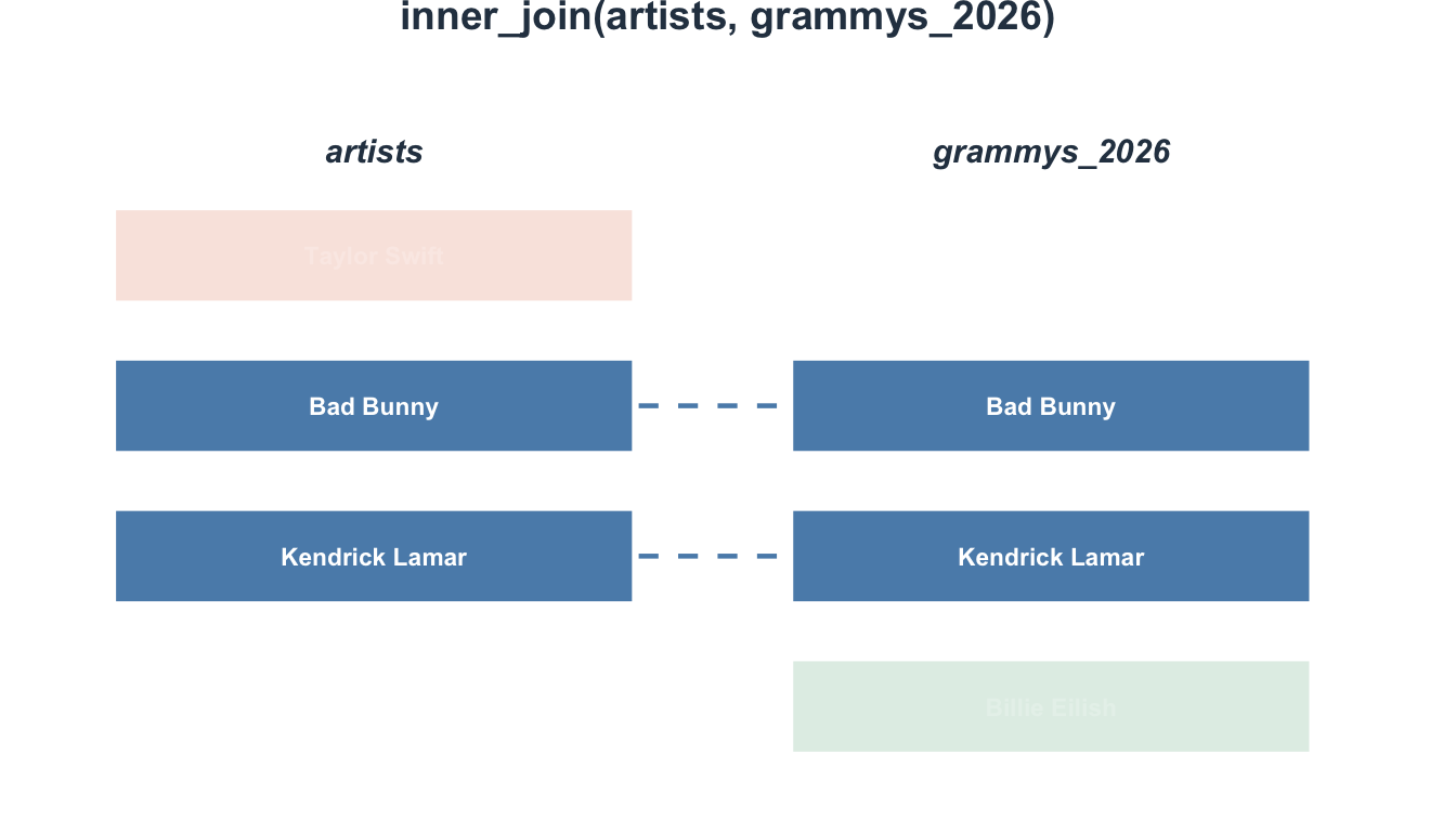
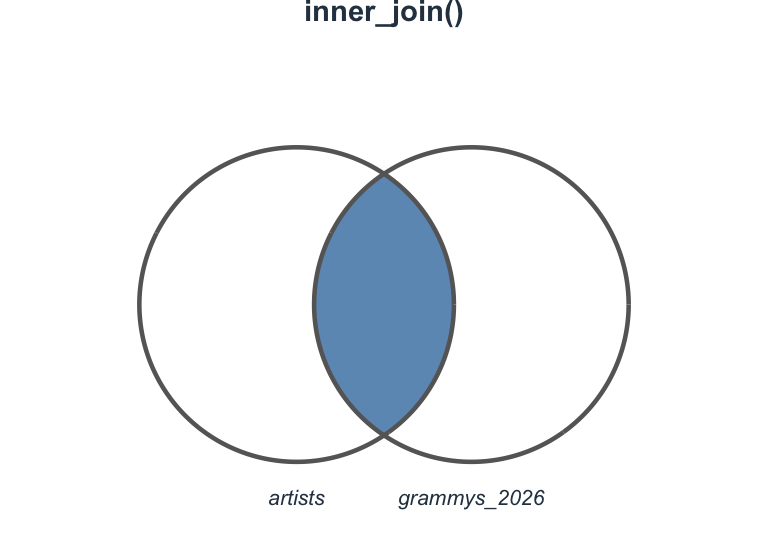
inner_join(): Only matches

Keep only rows that exist in both tables:

participants |>
  inner_join(survey, by = "participant_id")

# A tibble: 3 × 5
  participant_id   age condition depression anxiety
           <dbl> <dbl> <chr>          <dbl>   <dbl>
1              1    22 Control           12      15
2              2    25 Treatment         18      20
3              3    19 Treatment         10      12

• Participant 4 excluded (no survey data)
• Participant 5 excluded (not in participants)

Emphasize that inner_join() silently drops rows that do not match, which means you lose data without a warning. In psychology research this is usually not what you want — you want to know who is missing, not hide them. This is why left_join() is the default recommendation. Students may ask “when would I actually use inner_join?” — a fair answer is when you only want to analyze people who completed both measures and you have already documented the attrition.

Visualizing inner_join()

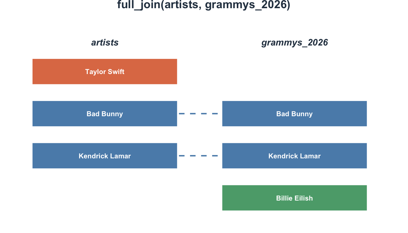
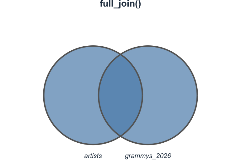
full_join(): Everything

Keep all rows from both tables:

participants |>
  full_join(survey, by = "participant_id")

# A tibble: 5 × 5
  participant_id   age condition depression anxiety
           <dbl> <dbl> <chr>          <dbl>   <dbl>
1              1    22 Control           12      15
2              2    25 Treatment         18      20
3              3    19 Treatment         10      12
4              4    31 Control           NA      NA
5              5    NA <NA>              25      30

Every participant appears, with NA where data is missing.

Point out that full_join() gives you the most complete picture — nobody is dropped. But it also means you may have rows with lots of NAs — exactly the kind of explicit missingness we discussed last session. Good moment to call back to drop_na(), replace_na(), and the “make implicit missing explicit” idea: full_join() does the same job, just for combining tables.

Visualizing full_join()

Join types at a glance

Which join should I use?

Most common in psychology: left_join()

Use when:

• You have a main participant table
• You want to add additional data (surveys, behavioral tasks)
• You want to keep all participants, even those with missing data

Tip

Start with left_join() unless you have a specific reason to use another type.

Reinforce this strongly: “If you remember nothing else from today, remember left_join().” In practice, 90% of joins students will do in this course and in research are left joins. The mental model is simple: “I have a main table and I want to stick more columns onto it.” Spend ~2 minutes here before transitioning to the psychology example.

Psychology example: Adding demographics

# Task data
task_data <- tibble(
  participant_id = c(1, 2, 3, 1, 2, 3),
  trial = c(1, 1, 1, 2, 2, 2),
  reaction_time = c(450, 380, 520, 430, 395, 510)
)

# Add participant info to each trial
task_data |>
  left_join(participants, by = "participant_id")

# A tibble: 6 × 5
  participant_id trial reaction_time   age condition
           <dbl> <dbl>         <dbl> <dbl> <chr>    
1              1     1           450    22 Control  
2              2     1           380    25 Treatment
3              3     1           520    19 Treatment
4              1     2           430    22 Control  
5              2     2           395    25 Treatment
6              3     2           510    19 Treatment

Draw attention to what happened to the row count. The task_data table has 6 rows (3 participants x 2 trials) and the participants table has 4 rows, but the result still has 6 rows. This is because left_join() matched each trial row to the participant’s demographics and repeated the demographic info for each trial. Students often expect the result to have more or fewer rows — this is a good moment to check their intuition.

Joining by multiple keys

Remember the longitudinal example earlier — participant_id repeated, but participant_id + timepoint was unique. Joins handle this too.

# Depression at two timepoints
depression_long <- tibble(
  id = c(1, 1, 2, 2),
  time = c(1, 2, 1, 2),
  depression = c(20, 15, 18, 12)
)

# Anxiety at the same timepoints
anxiety_long <- tibble(
  id = c(1, 1, 2, 2),
  time = c(1, 2, 1, 2),
  anxiety = c(14, 10, 16, 11)
)

Joining on id AND time

If we joined on id alone, each row in one table would match both timepoints in the other — wrong! We need to match on both columns:

depression_long |>
  left_join(anxiety_long, by = c("id", "time"))

# A tibble: 4 × 4
     id  time depression anxiety
  <dbl> <dbl>      <dbl>   <dbl>
1     1     1         20      14
2     1     2         15      10
3     2     1         18      16
4     2     2         12      11

Pass a vector of column names to by. R requires all of them to match.

This is the payoff for the compound-key idea from earlier in the deck — when one column does not uniquely identify a row, you join on multiple columns. Walk through what would happen if we used by = "id" alone: participant 1’s Time 1 depression would match both of participant 1’s anxiety rows (Time 1 and Time 2), doubling the output. The vector c("id", "time") tells dplyr to require BOTH columns to match. This is the syntax students will use any time longitudinal data is spread across files.

Pair coding break

Your turn: Combine study data

You have three tables from a therapy study:

baseline <- tibble(
  id = 1:5,
  age = c(25, 30, 22, 35, 28),
  baseline_depression = c(22, 25, 18, 30, 20)
)

treatment <- tibble(
  id = c(1, 2, 3, 4),  # Missing id 5
  condition = c("CBT", "Control", "CBT", "Control")
)

followup <- tibble(
  id = c(1, 2, 3, 5),  # Missing id 4, but has id 5
  followup_depression = c(12, 23, 10, 18)
)

Your turn: Combine study data

1. Create a dataset with baseline info and treatment condition (keep all participants)
2. Add followup data (keep all from step 1)
3. How many participants are missing followup data?

Time: 10 minutes

Circulate during the exercise. The most common mistake is using inner_join() instead of left_join(), which silently drops participant 5 in step 1. If pairs finish early, ask them to figure out which participants are missing followup data and whether missingness is related to condition. That bridges to the filtering joins section. When time is up, walk through the solution and emphasize step 3 — the sum(is.na()) pattern is the same one they used last session for missing data.

Solution: Combine study data

# Steps 1 & 2: Chain two left_joins — baseline is the "spine"
# so every participant is kept, even those missing later data.
alldata <- baseline |>
  left_join(treatment, by = "id") |>
  left_join(followup, by = "id")

alldata

# Step 3: How many are missing followup?
alldata |>
  summarize(
    miss_followup = sum(is.na(followup_depression))
  )

# Bonus: count NAs across every column at once
alldata |>
  summarize(
    across(
      everything(),
      ~sum(is.na(.))
    )
  )

Filtering joins

A different purpose

Filtering joins don’t add columns — they filter rows based on whether matches exist:

• semi_join() — Keep rows that have a match
• anti_join() — Keep rows that don’t have a match

Transition cue: “So far every join we have seen adds columns. Filtering joins are different — they only keep or remove rows.” Emphasize the contrast: mutating joins change the width of your table, filtering joins change the height. Students sometimes wonder why you would not just use filter() — the answer is that filtering joins let you filter based on whether a match exists in another table, which filter() alone cannot do.

semi_join(): Has a match

Keep rows from the left table that exist in the right table:

# Which participants completed the survey?
participants |>
  semi_join(survey, by = "participant_id")

# A tibble: 3 × 3
  participant_id   age condition
           <int> <dbl> <chr>    
1              1    22 Control  
2              2    25 Treatment
3              3    19 Treatment

Only participants 1, 2, and 3 completed the survey.

anti_join(): No match

Keep rows from the left table that don’t exist in the right table:

# Which participants didn't complete the survey?
participants |>
  anti_join(survey, by = "participant_id")

# A tibble: 1 × 3
  participant_id   age condition
           <int> <dbl> <chr>    
1              4    31 Control  

Participant 4 didn’t complete the survey.

Psychology use case: Attrition analysis

# Who was enrolled
enrolled <- tibble(
  participant_id = 1:10,
  condition = rep(c("Treatment", "Control"), each = 5))

# Who completed
completed <- tibble(
  participant_id = c(1, 2, 3, 4, 7, 8, 9, 10))  # Missing 5 and 6

# Who dropped out?
enrolled |>
  anti_join(completed, by = "participant_id")

# A tibble: 2 × 2
  participant_id condition
           <int> <chr>    
1              5 Treatment
2              6 Control  

This is the “aha” moment for anti_join(). Walk through it slowly: “enrolled has 10 people, completed has 8 — anti_join gives us the 2 who are in enrolled but not in completed.” This is exactly what psychologists need for attrition analyses, and students will use it on their final projects if they have longitudinal or multi-session data. Linger on this example — it is more memorable than the abstract definition.

Attrition by condition

dropout <- enrolled |>
  anti_join(completed, by = "participant_id")

dropout |>
  count(condition)

# A tibble: 2 × 2
  condition     n
  <chr>     <int>
1 Control       1
2 Treatment     1

Warning

Both dropouts were from the Treatment condition — this could bias results!

This slide connects back to Session 1’s discussion of the replication crisis. If participants drop out of the treatment condition because the treatment is unpleasant, your remaining sample is biased — only the people who tolerated the treatment are left. This is differential attrition and it is a real threat to internal validity. Emphasize: “The code is simple, but the implication for your research is huge.”

Common join problems

Problem 1: Keys with different names

demographics <- tibble(
  subj_id = 1:3,
  age = c(25, 30, 22)
)

scores <- tibble(
  participant = c(1, 2, 3),
  depression = c(18, 22, 15)
)

Solution: Use named vector in by:

demographics |>
  left_join(scores,
    by = c("subj_id" = "participant"))

# A tibble: 3 × 3
  subj_id   age depression
    <dbl> <dbl>      <dbl>
1       1    25         18
2       2    30         22
3       3    22         15

This is the single most common join problem students will encounter with real data. Different labs, different Qualtrics surveys, different RA conventions — the ID column is almost never named the same thing across files. Remind them of the syntax: left table name on the left side of the equals sign, right table name on the right. If they forget the by argument entirely, R will try to join on all shared column names, which often produces wrong results silently.

Problem 2: Duplicate keys

# Duplicate in left table
participants_dup <- tibble(
  id = c(1, 1, 2, 3),  # ID 1 appears twice!
  age = c(25, 25, 30, 22)
)

task_scores <- tibble(
  id = c(1, 2, 3),
  score = c(85, 90, 88)
)

What happens with duplicates?

participants_dup |>
  left_join(task_scores, by = "id")

# A tibble: 4 × 3
     id   age score
  <dbl> <dbl> <dbl>
1     1    25    85
2     1    25    85
3     2    30    90
4     3    22    88

Each duplicate gets matched → creates extra rows!

Catch duplicates first

Use the same uniqueness check from earlier — before you join:

participants_dup |>
  count(id) |>
  filter(n > 1)

# A tibble: 1 × 2
     id     n
  <dbl> <int>
1     1     2

id = 1 appears twice. Now you can decide: is this longitudinal data (→ use a compound key) or a data-entry error (→ fix the data)?

This is the sneakiest bug students will encounter. The join runs without error, but you end up with more rows than expected. Students often do not notice until their summary statistics look wrong. Reinforce the habit: always run the count-and-filter check before joining. Ask: “If your table had 100 participants and after a join it has 105 rows, what happened?” Duplicates.

Problem 3: Missing keys

# Some participants have NA for id
messy_data <- tibble(
  id = c(1, 2, NA, 3),
  response = c("Yes", "No", "Yes", "No")
)

demographics <- tibble(
  id = 1:3,
  age = c(25, 30, 22)
)

Joining with NAs

messy_data |>
  left_join(demographics, by = "id")

# A tibble: 4 × 3
     id response   age
  <dbl> <chr>    <dbl>
1     1 Yes         25
2     2 No          30
3    NA Yes         NA
4     3 No          22

Row with NA id can’t match → gets NA for age.

Fix the data before joining!

Problem 4: Many-to-many relationships

# Multiple trials, nested within sessions
trials <- tibble(
  id      = c(1, 1, 1, 1, 2, 2, 2, 2),
  session = c(1, 1, 2, 2, 1, 1, 2, 2),
  trial   = c(1, 2, 1, 2, 1, 2, 1, 2),
  rt      = c(450, 430, 460, 440, 380, 390, 375, 385)
)

# Mood reported once per session
session_mood <- tibble(
  id      = c(1, 1, 2, 2),
  session = c(1, 2, 1, 2),
  mood    = c(5, 6, 4, 5)
)

What goes wrong

# Joining on id alone — each trial matches every session for that id
trials |>
  left_join(session_mood, by = "id")

# A tibble: 16 × 6
      id session.x trial    rt session.y  mood
   <dbl>     <dbl> <dbl> <dbl>     <dbl> <dbl>
 1     1         1     1   450         1     5
 2     1         1     1   450         2     6
 3     1         1     2   430         1     5
 4     1         1     2   430         2     6
 5     1         2     1   460         1     5
 6     1         2     1   460         2     6
 7     1         2     2   440         1     5
 8     1         2     2   440         2     6
 9     2         1     1   380         1     4
10     2         1     1   380         2     5
11     2         1     2   390         1     4
12     2         1     2   390         2     5
13     2         2     1   375         1     4
14     2         2     1   375         2     5
15     2         2     2   385         1     4
16     2         2     2   385         2     5

8 trials became 16 rows. The join silently created all combinations.

Fix: use a compound key

trials |>
  left_join(session_mood, by = c("id", "session"))

# A tibble: 8 × 5
     id session trial    rt  mood
  <dbl>   <dbl> <dbl> <dbl> <dbl>
1     1       1     1   450     5
2     1       1     2   430     5
3     1       2     1   460     6
4     1       2     2   440     6
5     2       1     1   380     4
6     2       1     2   390     4
7     2       2     1   375     5
8     2       2     2   385     5

Now each trial matches the mood from its own session — back to 8 rows.

Many-to-many joins are the sneakiest mistake students will make with real data. The join runs without an error — but the row count explodes. Always sanity-check: if you joined an 8-row table with a 4-row table and got 16 rows, something is off. The fix is almost always to add another column to the by argument so the match becomes unique. This is the same compound-key idea from the longitudinal join earlier in the deck.

Practical psychology examples

Example 1: Qualtrics + demographics

# Survey responses exported from Qualtrics
qualtrics <- tibble(
  ResponseId = c("R_1", "R_2", "R_3"),
  PHQ9_total = c(12, 18, 8),
  GAD7_total = c(10, 15, 6)
)

# Demographics collected separately
demo <- tibble(
  ResponseId = c("R_1", "R_2", "R_3"),
  age = c(25, 30, 22),
  major = c("Psychology", "Sociology", "Psychology")
)

Transition cue: “Let me show you three examples of how this works with real psychology workflows.” The Qualtrics example is the most immediately relevant for students who are running their own studies. Mention that Qualtrics exports include ResponseId automatically, which makes it a natural join key when you have separate survey blocks exported as different CSVs.

Example 1: Result

qualtrics |>
  left_join(demo, by = "ResponseId")

# A tibble: 3 × 5
  ResponseId PHQ9_total GAD7_total   age major     
  <chr>           <dbl>      <dbl> <dbl> <chr>     
1 R_1                12         10    25 Psychology
2 R_2                18         15    30 Sociology 
3 R_3                 8          6    22 Psychology

Example 2: Pre-post intervention

pre_test <- tibble(
  participant = 1:4,
  depression_pre = c(22, 25, 18, 20)
)

post_test <- tibble(
  participant = c(1, 2, 4),  # 3 dropped out
  depression_post = c(12, 23, 15)
)

Example 2: Result

# Combine and compute change
pre_test |>
  left_join(post_test, by = "participant") |>
  mutate(change = depression_pre - depression_post)

# A tibble: 4 × 4
  participant depression_pre depression_post change
        <dbl>          <dbl>           <dbl>  <dbl>
1           1             22              12     10
2           2             25              23      2
3           3             18              NA     NA
4           4             20              15      5

Example 3: Item-level to scale-level

# Individual items
items <- tibble(
  id = rep(1:3, each = 5),
  item = rep(1:5, times = 3),
  response = c(3,4,3,4,3, 2,3,2,3,2, 4,5,4,5,4)
)

# Participant info
participants_info <- tibble(
  id = 1:3,
  condition = c("Control", "Treatment", "Treatment")
)

Example 3: Result

# Compute scale scores then join
items |>
  group_by(id) |>
  summarize(scale_mean = mean(response)) |>
  left_join(participants_info, by = "id")

# A tibble: 3 × 3
     id scale_mean condition
  <int>      <dbl> <chr>    
1     1        3.4 Control  
2     2        2.4 Treatment
3     3        4.4 Treatment

This example shows a common pattern: summarize first, then join. Students often try to join first and then summarize, which can work but is harder to reason about (especially if the join changes the number of rows). Encourage the “reduce then combine” workflow: compute your scale scores, then attach the metadata. This is also a nice callback to the group_by + summarize skills from earlier in the course.

End-of-deck exercise

Practice: Longitudinal study

This exercise is a head start on Assignment 7 (Joins and Missing Data). It combines multiple join types — left_join for building the dataset, anti_join for identifying dropout — and asks students to think about attrition patterns. Give them ~10 minutes. If they get stuck on task 3 (identifying dropout at each wave), hint that anti_join is the right tool. Task 4 (dropout by condition) is the stretch goal; do not worry if not everyone gets there.

You have data from a three-wave longitudinal study:

# Baseline demographics
baseline_demo <- tibble(
  pid = 1:6,
  age = c(20, 22, 25, 19, 24, 21),
  condition = rep(c("Intervention", "Control"), each = 3)
)

# Time 1 assessment
time1_scores <- tibble(
  pid = 1:6,
  depression_t1 = c(22, 25, 18, 20, 24, 19)
)

# Time 2 assessment (2 dropouts)
time2_scores <- tibble(
  pid = c(1, 2, 3, 4, 6),  # Missing 5
  depression_t2 = c(15, 24, 12, 18, 17)
)

# Time 3 assessment (1 more dropout)
time3_scores <- tibble(
  pid = c(1, 2, 3, 6),  # Missing 4 and 5
  depression_t3 = c(12, 22, 10, 15)
)

Your tasks

1. Create a complete dataset with all timepoints
2. Compute change scores (T1 to T3)
3. Identify who dropped out at each wave
4. Check if dropout differs by condition

Solution: Longitudinal study

# 1. Build the complete dataset — baseline is the spine.
alldata2 <- baseline_demo |>
  left_join(time1_scores, by = "pid") |>
  left_join(time2_scores, by = "pid") |>
  left_join(time3_scores, by = "pid")

# 2. Change score from T1 to T3.
alldata2 <- alldata2 |>
  mutate(change = depression_t3 - depression_t1)

# 3a. Who dropped out at T2? (in baseline, missing from time2)
baseline_demo |>
  anti_join(time2_scores)

# 3b. Who dropped out at T3? Broken down by condition.
baseline_demo |>
  anti_join(time3_scores) |>
  count(condition)

# Bonus: who finished T2 but dropped before T3? Attach demographics
# to see who they are.
time2_scores |>
  anti_join(time3_scores) |>
  left_join(baseline_demo)

Wrapping up

Join decision flowchart

Ask yourself:

1. Do I want to add columns?
   • Yes → Use a mutating join
   • No → Use a filtering join
2. Which rows do I want to keep?
   • All from left → left_join()
   • All from right → right_join()
   • Only matches → inner_join()
   • Everything → full_join()

3. Am I filtering rows?
   • Keep matches → semi_join()
   • Keep non-matches → anti_join()

Walk through this flowchart as a decision tree. Consider having students practice with a quick verbal exercise: you describe a scenario and they call out which join to use. For example: “I want to add survey scores to my participant table” (left_join), “I want to find out which participants did NOT complete the follow-up” (anti_join). Two or three of these takes about 2 minutes and solidifies the mental model.

Key takeaways

1. Joins combine data from multiple tables using key variables
2. Check your keys for uniqueness before joining
3. left_join() is your workhorse — keeps all rows from your main table
4. Filtering joins help identify completers vs. dropouts
5. Watch for common problems: duplicate keys, different key names, NAs
6. Always inspect the result to ensure it matches expectations

Before next class

📖 Read:

• R4DS Ch 11: Communication

✅ Do:

• Finish Assignment 7 (due Sun May 24)
• Check if your final project needs joins
• Practice joining your own data files

The one thing to remember

If your data lives in separate files, joins are how you ask a question that spans all of them.

See you Wednesday for storytelling with data!

End strong on this takeaway. Remind students that Assignment 7 (Joins and Missing Data) is due Sunday May 24 — both halves of the assignment are now fair game. Note that Memorial Day is the following Monday so the next class is Wednesday May 27 (Storytelling with Data). The final project draft was due today, so they should now be working on cleaning and analyzing their own data with all the tools they’ve learned.