Missing Data

PSY 410: Data Science for Psychology

Dr. Sara Weston

2026-05-13

Why missing data matters

The data you don’t have

In a typical longitudinal psychology study, 30–50% of participants drop out before the final wave.

If you just delete their data, you might be throwing away the most important part of the story — because who drops out is rarely random.

Today we learn to detect, explore, and handle missing data honestly.

PACING (~80 min total): Why missing data matters (~5). Types of missing data (~8). Exploring missing data (~10). Handling missing data (~15). Implicit→explicit (~8). Pair coding (~10). Mechanisms + reporting (~12). Multiple imputation (~2). Wrap-up (~5). If running short, cut the multiple imputation section entirely and shorten the MCAR/MAR/MNAR examples — the reporting paragraph at the end is the more important takeaway.

A6 reminder: Make sure to flag at the top of class (and again at the end) that Assignment 6 is due Sunday May 17 at 11:59 PM — that’s this weekend, so it’s the most pressing deadline on their plate.

Ask if anyone ran into NAs while exploring data for their final project. The 30-50% statistic is a real number from attrition research and tends to surprise students. Emphasize the word “honestly” — this session is as much about research ethics and transparency as it is about R functions. Spend ~2 minutes on this opening.

Types of missing data

Explicit missing: NA

Explicit missing means you can see the NA:

survey <- tibble(
  participant = 1:5,
  age = c(25, NA, 30, 22, NA),
  depression = c(12, 18, NA, 10, 15)
)

survey

# A tibble: 5 × 3
  participant   age depression
        <int> <dbl>      <dbl>
1           1    25         12
2           2    NA         18
3           3    30         NA
4           4    22         10
5           5    NA         15

The NA values are obvious.

Students have seen NA before (it shows up whenever a function can’t compute a value, or when data is missing from a CSV), but this is the first time we treat it as a topic in its own right. Make sure they understand that NA means “we do not know” — not zero, not blank, not “no answer.” R treats NA differently from any other value, which is why things like NA == NA return NA, not TRUE. You do not need to go deep on that quirk, but mention it because students will stumble on it eventually.

Implicit missing: Rows don’t exist

Implicit missing means entire rows are absent:

appointments <- tibble(
  name = c("Alice", "Bob", "Alice", "Carol"),
  day = c("Mon", "Mon", "Wed", "Wed"),
  attended = c(TRUE, TRUE, TRUE, TRUE)
)

appointments

# A tibble: 4 × 3
  name  day   attended
  <chr> <chr> <lgl>   
1 Alice Mon   TRUE    
2 Bob   Mon   TRUE    
3 Alice Wed   TRUE    
4 Carol Wed   TRUE    

Who didn’t show up? You can’t tell because they’re not in the data!

This distinction (explicit vs. implicit) is one of the most important conceptual takeaways. Ask students: “Bob is not in the Wednesday data. Did he attend and the data was not recorded? Or did he not attend? Or did he cancel?” The data cannot tell us. This is much harder to detect than explicit NAs because there is nothing to see — the row simply does not exist. We will see complete() later in this deck as the main tool for surfacing implicit missingness within a single dataset.

Why implicit missing matters

In longitudinal studies, missing rows often mean dropout:

# Three-wave study
longitudinal <- tibble(
  id = c(1, 1, 1, 2, 2, 3),  # Person 2 missing wave 3, person 3 missing waves 2 and 3
  wave = c(1, 2, 3, 1, 2, 1),
  depression = c(20, 15, 12, 25, 22, 18)
)

longitudinal

# A tibble: 6 × 3
     id  wave depression
  <dbl> <dbl>      <dbl>
1     1     1         20
2     1     2         15
3     1     3         12
4     2     1         25
5     2     2         22
6     3     1         18

Person 2 and 3’s missing waves are implicit — they’re not NA, they’re just absent.

Exploring missing data

Checking for NAs

survey <- tibble(
  id = 1:6,
  age = c(25, NA, 30, 22, NA, 28),
  depression = c(12, 18, NA, 10, 15, NA),
  anxiety = c(15, 20, 12, NA, 18, 16)
)

# Check if any NAs exist
any(is.na(survey))

[1] TRUE

# Count total NAs
sum(is.na(survey))

[1] 5

Walk through these two functions as the first step in any missing-data analysis. The any() check is a quick yes/no diagnostic; sum() tells you the scale of the problem. Point out that is.na() returns TRUE/FALSE, and since R treats TRUE as 1 and FALSE as 0, sum() counts the TRUEs — a useful trick that recurs throughout the tidyverse.

NAs by column

# Count NAs in each column
survey |>
  summarize(
    age_missing = sum(is.na(age)),
    depression_missing = sum(is.na(depression)),
    anxiety_missing = sum(is.na(anxiety))
  )

# A tibble: 1 × 3
  age_missing depression_missing anxiety_missing
        <int>              <int>           <int>
1           2                  2               1

Better approach: across()

across(columns, function) applies the same function to multiple columns at once:

survey |>
  summarize(
    across(
      everything(),       # which columns: all of them
      ~ sum(is.na(.x))    # what to do: count NAs (.x = "this column")
    )
  )

# A tibble: 1 × 4
     id   age depression anxiety
  <int> <int>      <int>   <int>
1     0     2          2       1

The across() + everything() pattern is essentially new for most students — they only saw it briefly in Session 10 and were told to focus on output, not mechanics. Walk through the anatomy slowly: across() takes (1) which columns and (2) what to do to each. The tilde (~) plus .x is shorthand for “for each column, do this.” Spend ~3 minutes on this slide since the syntax is unfamiliar.

Or as proportions

survey |>
  summarize(
    across(
      everything(),
      ~ mean(is.na(.x))
    )
  )

# A tibble: 1 × 4
     id   age depression anxiety
  <dbl> <dbl>      <dbl>   <dbl>
1     0 0.333      0.333   0.167

Swapping sum() for mean() turns counts into proportions — a useful trick that reuses the TRUE = 1 / FALSE = 0 idea. This is especially useful for reporting: “33% of participants were missing age data.” Students often ask whether to report counts or proportions; the answer is both, ideally.

Visualizing missingness

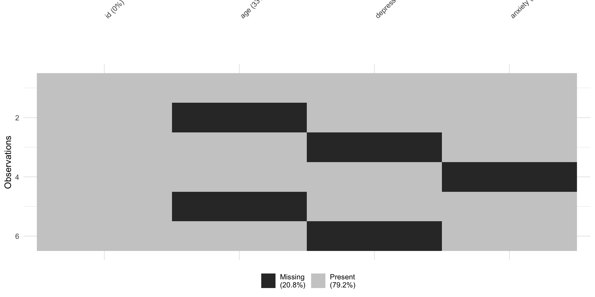
The naniar package provides great visualization tools:

library(naniar)

# Visual summary
vis_miss(survey)

The naniar package is optional — students do not need to install it for assignments. But the vis_miss() plot is a great diagnostic tool worth showing. Each column is a variable, each row is a participant, and missing cells are colored. This gives an immediate visual sense of where the holes are. If naniar is not installed on your machine, you can skip this live and just show the rendered output.

Handling missing data

Strategy 1: Complete case analysis

Complete case analysis (listwise deletion) removes any row with any NA:

survey |>
  drop_na()

# A tibble: 1 × 4
     id   age depression anxiety
  <int> <dbl>      <dbl>   <dbl>
1     1    25         12      15

Transition cue: “Now that we know how to find missing data, let’s talk about what to do about it.” Students often default to this strategy because it is the simplest — the next slide shows why that can be dangerous. (Aside, if students ever see na.omit() elsewhere: it’s the base R equivalent of drop_na() — same behavior.)

Dangers of complete case analysis

# Started with 6 participants
nrow(survey)

[1] 6

# Only 2 complete cases
survey |>
  drop_na() |>
  nrow()

[1] 1

Warning

You just lost 67% of your data!

Let this number land. Going from 6 to 2 participants is dramatic, and it gets worse with real datasets that have many variables — each additional variable with any missingness compounds the loss. In a study with 20 survey items, even a small per-item missing rate can reduce your sample to almost nothing if you use listwise deletion. Ask: “Would you trust a result based on 2 participants?” This motivates the selective dropping approach on the next slide.

Selective dropping

Only drop rows missing specific variables:

# Drop only if depression is missing
survey |>
  drop_na(depression)

# A tibble: 4 × 4
     id   age depression anxiety
  <int> <dbl>      <dbl>   <dbl>
1     1    25         12      15
2     2    NA         18      20
3     4    22         10      NA
4     5    NA         15      18

Drop on multiple variables

# Drop only if depression OR anxiety is missing
survey |>
  drop_na(depression, anxiety)

# A tibble: 3 × 4
     id   age depression anxiety
  <int> <dbl>      <dbl>   <dbl>
1     1    25         12      15
2     2    NA         18      20
3     5    NA         15      18

When is dropping okay?

Dropping is fine when:

• Missing data is rare (< 5-10%)
• Missingness is truly random
• You have adequate sample size

Be cautious when:

• Missing data is common (> 20%)
• Certain groups have more missingness (systematic bias)
• Sample size is small

The 5-10% and 20% thresholds are rules of thumb, not hard cutoffs. The key question is always “does the missingness bias my results?” If depressed people are the ones skipping the depression questionnaire, then even 5% missing data is a problem. Emphasize that the amount of missing data matters less than the pattern. This sets up the MCAR/MAR/MNAR discussion later in the deck.

Strategy 2: Filling values

Sometimes you can reasonably fill missing values:

# Carry forward the last observation
time_series <- tibble(
  day = 1:5,
  mood = c(5, NA, NA, 4, 6)
)

time_series |>
  fill(mood)  # Fills downward by default

# A tibble: 5 × 2
    day  mood
  <int> <dbl>
1     1     5
2     2     5
3     3     5
4     4     4
5     5     6

fill() is called “last observation carried forward” (LOCF) in clinical research. It assumes the missing values are the same as the most recent non-missing value. This is reasonable for things like demographic variables that do not change between rows (e.g., filling in a participant’s age across multiple trials), but more questionable for outcome variables. Students often want to use fill() for everything — the warning slide that follows is important.

Fill directions

# Fill upward
time_series |>
  fill(mood, .direction = "up")

# A tibble: 5 × 2
    day  mood
  <int> <dbl>
1     1     5
2     2     4
3     3     4
4     4     4
5     5     6

When is filling okay?

Filling makes sense for:

• Time series with repeated measures (carry forward last observation)
• Grouping variables that apply to multiple rows
• Values that don’t change often

Warning

NEVER fill when it means making up data you don’t have!

Strategy 3: Replace with a specific value

# Replace NAs with a value
survey |>
  mutate(
    age = replace_na(age, 99),  # Code 99 = "no response"
    depression = replace_na(depression, -999)  # Obvious invalid code
  )

# A tibble: 6 × 4
     id   age depression anxiety
  <int> <dbl>      <dbl>   <dbl>
1     1    25         12      15
2     2    99         18      20
3     3    30       -999      12
4     4    22         10      NA
5     5    99         15      18
6     6    28       -999      16

Students often ask “why not just replace NA with the mean?” Replacing with the mean is a form of imputation that shrinks variance and can bias results — it is generally not recommended in modern practice. The placeholder codes shown here (99, -999) are a SPSS-era convention for marking missing data that should not be analyzed. If you use them, you must filter them out before computing any statistics. Generally, leaving values as NA is safer and more transparent.

Strategy 3: Replace with a specific value

Important

If you use placeholder codes, document them clearly and make sure they can’t be mistaken for real data.

Strategy 4: Leave them as NA

Often the best approach is to keep NAs and handle them in analysis:

# Most functions have na.rm argument
survey |>
  summarize(
    mean_age = mean(age, na.rm = TRUE),
    mean_depression = mean(depression, na.rm = TRUE)
  )

# A tibble: 1 × 2
  mean_age mean_depression
     <dbl>           <dbl>
1     26.2            13.8

This is transparent about what data you have.

Emphasize that this is often the best default for students at this level. Keeping NAs and using na.rm = TRUE is honest and simple. Remind them that without na.rm = TRUE, mean() will return NA if any values are missing — this is R’s way of saying “I cannot give you a trustworthy answer with incomplete data.” Students frequently forget na.rm and get confused by NA results; this is the fix.

Implicit missing → Explicit missing

The problem with implicit missing

study_completion <- tibble(
  participant = c(1, 1, 1, 2, 2, 3, 3),
  timepoint = c(1, 2, 3, 1, 2, 1, 3),
  depression = c(20, 15, 12, 25, 22, 18, 14)
)

study_completion

# A tibble: 7 × 3
  participant timepoint depression
        <dbl>     <dbl>      <dbl>
1           1         1         20
2           1         2         15
3           1         3         12
4           2         1         25
5           2         2         22
6           3         1         18
7           3         3         14

Who’s missing which timepoints? Hard to tell.

complete(): Make implicit missing explicit

study_completion |>
  complete(participant, timepoint)

# A tibble: 9 × 3
  participant timepoint depression
        <dbl>     <dbl>      <dbl>
1           1         1         20
2           1         2         15
3           1         3         12
4           2         1         25
5           2         2         22
6           2         3         NA
7           3         1         18
8           3         2         NA
9           3         3         14

Now we can see: Participant 2 missing timepoint 3, Participant 3 missing timepoint 2.

complete() is the key function for this section. It generates every combination of the variables you specify and fills in NA where data is missing. Walk through the output carefully: the original data had 7 rows, but with 3 participants and 3 timepoints there should be 9 rows. The 2 new rows (with NAs for depression) represent the implicit missing data that is now explicit. complete() is the cleanest way to surface implicit missingness within a single dataset — one function generates the grid and exposes the gaps.

Why this matters

Makes dropout visible for analysis:

study_completion |>
  complete(participant, timepoint) |>
  group_by(timepoint) |>
  summarize(
    n_completed = sum(!is.na(depression)),
    n_missing = sum(is.na(depression))
  )

# A tibble: 3 × 3
  timepoint n_completed n_missing
      <dbl>       <int>     <int>
1         1           3         0
2         2           2         1
3         3           2         1

Flagging completion

Common pattern: make implicit explicit, then flag who completed each timepoint:

study_completion |>
  complete(participant, timepoint) |>
  mutate(
    completed = if_else(is.na(depression), FALSE, TRUE)
  )

# A tibble: 9 × 4
  participant timepoint depression completed
        <dbl>     <dbl>      <dbl> <lgl>    
1           1         1         20 TRUE     
2           1         2         15 TRUE     
3           1         3         12 TRUE     
4           2         1         25 TRUE     
5           2         2         22 TRUE     
6           2         3         NA FALSE    
7           3         1         18 TRUE     
8           3         2         NA FALSE    
9           3         3         14 TRUE     

This completed flag is the building block for attrition analysis — coming up later in the deck.

Pair coding break

Your turn: Analyze missing data patterns

You have survey data from a therapy study:

therapy_survey <- tibble(
  id = 1:8,
  age = c(25, 30, NA, 22, 28, NA, 35, 26),
  baseline_depression = c(22, 25, 18, 20, 24, 19, NA, 21),
  followup_depression = c(12, 23, NA, 15, NA, NA, NA, 16),
  satisfaction = c(4, 3, NA, 5, 4, NA, NA, 5)
)

1. How many participants are missing baseline data? Followup data?
2. How many participants have complete data (no NAs anywhere)?
3. Create a version that drops rows missing followup data
4. What percentage of participants completed the followup?

Time: 10 minutes

Circulate during the exercise. For question 1, students can use sum(is.na()) or the across() approach — either is fine. The most common mistake on question 3 is using drop_na() without specifying the column, which drops too many rows. Question 4 is the most interesting: mean(!is.na(followup_depression)) gives the completion rate directly. When reviewing, connect this to reporting: “You would write something like ‘50% of participants completed the follow-up assessment.’”

Solution: Missing data patterns

# 1. NAs in every column at once — across() applies sum(is.na(.))
#    to each variable so we don't have to name them one by one.
therapy_survey |>
  summarize(
    across(everything(), ~sum(is.na(.x)))
  )

# 2. Complete cases — drop_na() with no arguments removes any row
#    that has an NA anywhere. nrow() then counts what's left.
therapy_survey |>
  drop_na() |>
  nrow()

# 3. Drop only rows missing followup — pass the column name to drop_na().
therapy_survey |>
  drop_na(followup_depression)

# 4. Completion rate — !is.na() flips the logic to "has a value",
#    and mean() of a TRUE/FALSE vector gives the proportion.
therapy_survey |>
  summarize(
    completion_rate = mean(!is.na(followup_depression))
  )

Psychology-specific considerations

Missing data mechanisms

Statisticians distinguish three types:

1. MCAR (Missing Completely At Random) — Missingness unrelated to anything
2. MAR (Missing At Random) — Missingness related to observed variables
3. MNAR (Missing Not At Random) — Missingness related to the missing value itself

This is conceptual — students do not need to memorize the acronyms, but they need to understand the core idea: the reason data is missing affects whether your results are biased. Spend ~5 minutes on this slide and the next two. The names are counterintuitive (especially MAR, which sounds like it should be unproblematic but actually means missingness is related to other measured variables). Use the depression study examples on the next slide to make each type concrete.

Example: Depression study

MCAR: Computer randomly failed to save 5% of responses

• No bias introduced

MAR: Older participants more likely to skip online surveys

• Can account for this by including age as a predictor

MNAR: People with severe depression skip the depression questionnaire

• This is a problem — missing values are related to what you’re measuring

Why it matters

• MCAR: Complete case analysis is fine (but you lose power)
• MAR: More sophisticated methods can help (beyond this course)
• MNAR: No easy fix — missing data is fundamentally informative

Tip

Your job: Always document and report how much data is missing and why you think it’s missing.

The practical takeaway for this course: you cannot statistically test whether data is MNAR (because you do not have the missing values to compare). So the best you can do is (1) document how much is missing, (2) check whether missingness is related to observed variables, and (3) be transparent about your assumptions. For their final projects, students should include a short paragraph about missing data even if they have very little — that is good practice.

Attrition analysis

In longitudinal studies, always check who drops out:

study <- tibble(
  id = 1:10,
  condition = rep(c("Treatment", "Control"), each = 5),
  baseline_depression = c(22, 18, 25, 20, 24, 19, 21, 23, 17, 22),
  followup_depression = c(15, 12, NA, NA, NA, 14, 13, 11, 16, 18)
)

study

# A tibble: 10 × 4
      id condition baseline_depression followup_depression
   <int> <chr>                   <dbl>               <dbl>
 1     1 Treatment                  22                  15
 2     2 Treatment                  18                  12
 3     3 Treatment                  25                  NA
 4     4 Treatment                  20                  NA
 5     5 Treatment                  24                  NA
 6     6 Control                    19                  14
 7     7 Control                    21                  13
 8     8 Control                    23                  11
 9     9 Control                    17                  16
10    10 Control                    22                  18

A missing followup score = a dropout.

This whole section is about applying the missing-data lens — is.na(followup_depression) identifies dropouts directly. Walk through the data: rows 3, 4, 5 are missing followup. Rows 1–5 are Treatment, so all three dropouts are in the Treatment condition. Set up the next slide as: “let’s confirm that programmatically.”

Who dropped out?

study |>
  filter(is.na(followup_depression))

# A tibble: 3 × 4
     id condition baseline_depression followup_depression
  <int> <chr>                   <dbl>               <dbl>
1     3 Treatment                  25                  NA
2     4 Treatment                  20                  NA
3     5 Treatment                  24                  NA

Dropout by condition

study |>
  filter(is.na(followup_depression)) |>
  count(condition)

# A tibble: 1 × 2
  condition     n
  <chr>     <int>
1 Treatment     3

All dropouts are from the Treatment condition — this could seriously bias results!

This is the punchline. If treatment dropouts are systematically different from completers (e.g., the treatment was unpleasant for some subset), then comparing post-treatment scores between conditions is comparing the people who tolerated the treatment to the full Control group — apples to oranges. Tie this to the MNAR discussion: this is exactly the kind of pattern that creates serious bias.

Reporting missing data

In your write-up, report:

1. How much data is missing (by variable)
2. Patterns of missingness (related to other variables?)
3. How you handled it (dropped? kept as NA?)
4. Potential biases (who’s missing? does it matter?)

Example:

“Eight participants (12%) did not complete the follow-up assessment. Dropout was unrelated to baseline depression scores (t = 1.2, p = .24). Analyses used complete case analysis (N = 60).”

Read the example paragraph aloud. This is the kind of reporting students should aim for in their final projects — at minimum, the count and percentage of missing data and a statement about how they handled it. They are not expected to run inferential tests for this course; the t-test in the example is just to show what a published version of this paragraph might look like. If a student asks how to test whether dropout is related to a categorical variable like condition (as we just demoed), the standard tool is a chi-squared test of independence — but it is well outside the scope of this course. This connects back to Session 1 and Session 16 themes about transparency and reproducibility.

Advanced topic: Multiple imputation

Beyond this course

More sophisticated approaches exist for handling missing data:

• Multiple imputation — create multiple plausible versions of missing data
• Maximum likelihood — estimate parameters using all available data
• Bayesian methods — incorporate uncertainty about missing values

Packages in R: mice, Amelia, missForest

Note

We won’t cover these methods, but know they exist for when you need them in future research!

Keep this brief — ~2 minutes. The goal is awareness, not instruction. Students who go on to graduate school will encounter these methods in statistics courses. For now, just knowing the names exist is enough. If a student asks for more detail, suggest they look at the mice package vignette after the course.

Wrapping up

Decision tree for missing data

1. How much is missing?
   • < 5%: Usually safe to drop
   • 5-20%: Investigate patterns
   • > 20%: Be very careful
2. Why is it missing?
   • Random: Less concerning
   • Systematic: Potentially biasing

3. What’s your plan?
   • Drop complete cases?
   • Drop specific variables?
   • Keep as NA and use na.rm?
   • Fill (carefully)?
4. Document everything!

Key takeaways

1. Missing data is normal in psychology research
2. Explicit vs implicit missing — make implicit explicit with complete()
3. Explore patterns before deciding how to handle
4. Complete case analysis (dropping rows) is simple but can lose power
5. Never make up data — be transparent about missingness
6. Document your decisions — report what’s missing and why
7. Check for bias — does missingness relate to key variables?

Functions cheat sheet

Function	Purpose
is.na()	Check if values are missing
drop_na()	Remove rows with NAs
replace_na()	Replace NAs with a value
fill()	Fill NAs with nearby values
complete()	Make implicit missing explicit
na.omit()	Remove rows with NAs (base R)
naniar::vis_miss()	Visualize missing data

Before next class

📖 Read:

• R4DS Ch 19: Joins

✅ Do:

• ⚠️ Finish Assignment 6 — due Sunday May 17 at 11:59 PM
• Start Assignment 7 — the missing-data half is fair game now
• Submit your final project draft (due next Wednesday before class)
• Check your own final project data for missingness

The one thing to remember

Missing data isn’t a problem to solve — it’s information about your study. Treat it that way.

See you Wednesday for joins!

End on this reframe. Students tend to think of NAs as a nuisance to get rid of. The takeaway is that missing data tells you something — about your study design, your participants, and potentially about your results.

Three deadlines to call out by name: 1. Assignment 6 is due Sunday May 17 at 11:59 PM — that’s the most pressing. Linger on this one — it’s only 4 days away. 2. Assignment 7 (Joins + Missing Data) was assigned today, due Sunday May 24. Tell them the missing-data half is doable now; joins comes Wednesday. 3. Final project draft (not the final report) is due next Wednesday May 20 before class.

Next session covers joins, which pairs naturally with missing data — joins are a major source of NAs.

The on-your-own exercise that follows is a take-home practice — point students to it but do not work through it in class.

On your own

Practice: Longitudinal missing data

This is a take-home exercise — students do not need to finish it in class. It focuses entirely on the missing-data tools from today (no joins yet — that’s next session). Task 1 uses complete(), tasks 2-3 combine summarize and filter with missing data logic, and task 4 reshapes wide and computes a change score. If they get stuck on task 4 in office hours, remind them: pivot_wider (Session 5) takes them from one-row-per-observation to one-row-per-participant, which is what they need for a wave-1-vs-wave-3 comparison. This exercise is directly relevant to Assignment 7.

You have a three-wave study:

longitudinal_study <- tibble(
  participant = c(1, 1, 1, 2, 2, 3, 3, 3, 4, 4),
  wave = c(1, 2, 3, 1, 2, 1, 2, 3, 1, 3),
  depression = c(25, 20, 15, 30, 28, 22, 18, 16, 20, NA),
  anxiety = c(28, 25, 22, 32, NA, 24, 20, 18, 22, 19)
)

Your tasks

1. Make implicit missing waves explicit using complete()
2. Count how many assessments each participant completed
3. What percentage of participants completed all three waves?
4. Reshape the depression data so each participant has one row with columns for wave 1, 2, and 3. Then compute the wave-1-to-wave-3 change for participants with both timepoints. What’s the mean change?

Solution: Longitudinal missing data

# 1. Make implicit missing explicit. complete() generates every
#    participant x wave combination and fills in NA where data
#    is absent — surfacing dropout that was hidden in the rows.
long_complete <- longitudinal_study |>
  complete(participant, wave)

long_complete

# 2. Count assessments per person — !is.na() is TRUE when a
#    score exists, and sum() counts those TRUEs.
long_complete |>
  group_by(participant) |>
  summarize(
    n_assessments = sum(!is.na(depression))
  )

# 3. Percentage who completed all 3 waves — a two-step summarize:
#    first count per participant, then take the mean of the
#    logical "n_assessments == 3" to get a proportion.
long_complete |>
  group_by(participant) |>
  summarize(
    n_assessments = sum(!is.na(depression))
  ) |>
  summarize(
    pct_complete = mean(n_assessments == 3)
  )

# 4. Reshape wide for a per-participant view, then compute change.
#    pivot_wider() gives one row per person with wave_1/2/3 columns;
#    filter() keeps only those with both wave 1 and wave 3 so the
#    subtraction is well-defined.
long_complete |>
  select(participant, wave, depression) |>
  pivot_wider(
    names_from = wave,
    values_from = depression,
    names_prefix = "wave_"
  ) |>
  filter(!is.na(wave_1) & !is.na(wave_3)) |>
  mutate(change = wave_1 - wave_3) |>
  summarize(mean_change = mean(change))