Data Tidying

PSY 410: Data Science for Psychology

Dr. Sara Weston

2026-04-13

What is tidy data?

Can you plot this?

participant	depression_pre	depression_post	anxiety_pre	anxiety_post
P1	18	12	24	20
P2	22	14	19	15
P3	15	11	28	22

Not easily. The columns mix variables (depression vs anxiety) with time points (pre vs post). ggplot doesn’t know what to put on each axis.

By the end of today, you’ll be able to reshape this into a form that works — and understand why it needs reshaping.

Open by showing this table and asking the class: “If I wanted to make a line graph of pre vs. post scores, what goes on the x-axis? What goes on the y-axis?” Let them struggle for a moment — the confusion is the point. This motivates the entire session. Spend ~2 minutes here.

The tidyverse philosophy

“Tidy datasets are all alike, but every messy dataset is messy in its own way.” — Hadley Wickham

The tools we’ve learned (ggplot2, dplyr) expect data in a specific format: tidy data.

The three rules of tidy data

1. Each variable is a column
2. Each observation is a row
3. Each value is a cell

Simple in theory, surprisingly complex in practice.

Spend ~3 minutes on the three rules. Have students say them aloud or repeat them back. The hardest part is rule 1 — students struggle with what counts as a “variable” vs. a “value.” Emphasize that this isn’t about right vs. wrong; it’s about what structure makes analysis easiest. You’ll come back to the “what is a variable?” question throughout the deck.

Tidy data visualized

Is this tidy?

participant	pre_test	post_test
P1	45	62
P2	52	58
P3	48	71

No! Time (pre/post) is a variable, but it’s spread across columns.

Pause before revealing the answer and poll the class: “Is this tidy?” Many students will say yes because it looks clean and organized. That’s a great teaching moment — tidy doesn’t mean “neat.” Emphasize that pre_test and post_test are values of a time variable, not separate variables.

The tidy version

Now it’s tidy!

participant	time	score
P1	pre	45
P1	post	62
P2	pre	52
P2	post	58
P3	pre	48
P3	post	71

Now: participant, time, and score are all columns.

Why does it matter?

Tidy data works with tidyverse tools:

# Easy to visualize
ggplot(data, aes(x = time, y = score, color = participant)) +
  geom_point()

# Easy to analyze
data |>
  group_by(time) |>
  summarize(mean = mean(score))

Connect this back to Sessions 2–4. Students already know ggplot and dplyr — point out that those tools assume tidy data. If their data isn’t tidy, the code they’ve already learned won’t work. This is the practical motivation: you’re not reshaping for fun, you’re reshaping so your tools work.

Wide vs. Long

Wide format

• Variables spread across columns
• One row per subject
• Humans like to read this

Long format

• Variables in a single column
• Multiple rows per subject
• R likes to work with this

Most real data needs reshaping.

Students often ask: “So wide is always wrong?” No — wide is fine for reading and some analyses. The key message is that most tidyverse tools expect long format, so you need to know how to get there. SPSS users especially will be used to wide format (one row per participant). Acknowledge that wide feels more natural to read, but long is what R needs.

Common untidy patterns

Pattern 1: Column headers are values

wide_scores <- tibble(
  student = c("Alice", "Bob", "Carol"),
  fall_2024 = c(85, 78, 92),
  spring_2025 = c(88, 82, 95),
  fall_2025 = c(91, 85, 94)
)
wide_scores

# A tibble: 3 × 4
  student fall_2024 spring_2025 fall_2025
  <chr>       <dbl>       <dbl>     <dbl>
1 Alice          85          88        91
2 Bob            78          82        85
3 Carol          92          95        94

The semester names are values, not variable names.

This is by far the most common untidy pattern in psychology data. Walk through this example slowly and ask: “What are the actual variables here?” (student, semester, score). The semester names are values of a semester variable, not variables in themselves. This is the pattern that pivot_longer() fixes. Spend ~2 minutes here; the next two patterns can be faster.

Pattern 2: Multiple variables in one column

messy_data <- tibble(
  id = 1:3,
  age_sex = c("25_M", "32_F", "28_F")
)
messy_data

# A tibble: 3 × 2
     id age_sex
  <int> <chr>  
1     1 25_M   
2     2 32_F   
3     3 28_F   

Age and sex are crammed into one column.

Pattern 3: Variables in rows and columns

weather <- tibble(
  id = c("MX001", "MX001", "MX002", "MX002"),
  year = c(2020, 2020, 2020, 2020),
  month = c(1, 2, 1, 2),
  element = c("tmax", "tmax", "tmin", "tmin"),
  value = c(85, 87, 32, 35)
)
weather

# A tibble: 4 × 5
  id     year month element value
  <chr> <dbl> <dbl> <chr>   <dbl>
1 MX001  2020     1 tmax       85
2 MX001  2020     2 tmax       87
3 MX002  2020     1 tmin       32
4 MX002  2020     2 tmin       35

element contains variable names (tmax, tmin).

Psychology-specific patterns

Surveys often look like:

survey_wide <- tibble(
  participant = 1:3,
  bdi_1 = c(2, 1, 3),
  bdi_2 = c(1, 0, 2),
  bdi_3 = c(3, 2, 2),
  bdi_4 = c(2, 1, 1)
)
survey_wide

# A tibble: 3 × 5
  participant bdi_1 bdi_2 bdi_3 bdi_4
        <int> <dbl> <dbl> <dbl> <dbl>
1           1     2     1     3     2
2           2     1     0     2     1
3           3     3     2     2     1

Each item is a column — wide format.

This is the example that will matter most for their assignments and thesis work. Point out that every Qualtrics export looks like this — one column per item. This dataset (survey_wide) will be reused in the pair coding exercise, so make sure students follow it. Transition: “Now let’s learn the function that fixes this.”

pivot_longer()

The most common tidying operation

pivot_longer() takes wide data and makes it long:

wide_scores |>
  pivot_longer(
    cols = fall_2024:fall_2025,  # Which columns to pivot
    names_to = "semester",        # New column for old column names
    values_to = "score"           # New column for values
  )

# A tibble: 9 × 3
  student semester    score
  <chr>   <chr>       <dbl>
1 Alice   fall_2024      85
2 Alice   spring_2025    88
3 Alice   fall_2025      91
4 Bob     fall_2024      78
5 Bob     spring_2025    82
6 Bob     fall_2025      85
7 Carol   fall_2024      92
8 Carol   spring_2025    95
9 Carol   fall_2025      94

This is the most important slide in the deck. Walk through each argument slowly, pointing at the output as you explain. Key confusion point: students mix up names_to and values_to. Use this mnemonic — “names_to is where the old column NAMES go; values_to is where the old cell VALUES go.” Run the code live so students see the output build. Spend ~3-4 minutes here.

Breaking it down

pivot_longer(
  cols = ...,        # Columns to reshape (use select helpers!)
  names_to = "...",  # Name for the new "names" column
  values_to = "..."  # Name for the new "values" column
)

Emphasize that names_to and values_to take quoted strings (these are new column names you are inventing). Students will forget the quotes — it’s one of the most common errors. Also note that cols uses the same selection syntax they learned in select(), which helps it feel less foreign.

Selecting columns to pivot

Use any of the select() helpers:

# By name
pivot_longer(cols = c(fall_2024, spring_2025, fall_2025))

# By range
pivot_longer(cols = fall_2024:fall_2025)

# By pattern
pivot_longer(cols = starts_with("fall"))
pivot_longer(cols = contains("202"))

# Everything except
pivot_longer(cols = -student)

Highlight the “everything except” pattern (cols = -student) — in practice, this is what students will use most often. When you have 50 BDI items and one ID column, you don’t want to list all 50 items. The negative selection is the practical shortcut.

Psychology example: Survey items

survey_wide |>
  pivot_longer(
    cols = starts_with("bdi"),
    names_to = "item",
    values_to = "response"
  )

# A tibble: 12 × 3
   participant item  response
         <int> <chr>    <dbl>
 1           1 bdi_1        2
 2           1 bdi_2        1
 3           1 bdi_3        3
 4           1 bdi_4        2
 5           2 bdi_1        1
 6           2 bdi_2        0
 7           2 bdi_3        2
 8           2 bdi_4        1
 9           3 bdi_1        3
10           3 bdi_2        2
11           3 bdi_3        2
12           3 bdi_4        1

Now each response is its own row!

Extracting information from names

What if column names contain useful info? We want to extract the time point (t1, t2, t3).

# Scores at different time points
experiment_wide <- tibble(
  id = 1:3,
  score_t1 = c(100, 95, 110),
  score_t2 = c(105, 100, 115),
  score_t3 = c(108, 102, 120)
)
experiment_wide

# A tibble: 3 × 4
     id score_t1 score_t2 score_t3
  <int>    <dbl>    <dbl>    <dbl>
1     1      100      105      108
2     2       95      100      102
3     3      110      115      120

names_prefix argument

experiment_wide |>
  pivot_longer(
    cols = starts_with("score"),
    names_to = "time",
    names_prefix = "score_",  # Remove this prefix from names
    values_to = "score"
  )

# A tibble: 9 × 3
     id time  score
  <int> <chr> <dbl>
1     1 t1      100
2     1 t2      105
3     1 t3      108
4     2 t1       95
5     2 t2      100
6     2 t3      102
7     3 t1      110
8     3 t2      115
9     3 t3      120

Without names_prefix, the time column would contain “score_t1”, “score_t2”, etc. — the full column name. That’s messy. names_prefix strips the redundant part, leaving clean values like “t1”, “t2”, “t3”. Students often forget this argument exists and try to fix the names afterward with mutate() + str_remove(). Mention that this is the cleaner approach.

names_pattern argument

For more complex parsing:

# Column names like "bdi_1", "anxiety_1", etc.
multi_scale <- tibble(
  id = 1:2,
  bdi_1 = c(2, 1), bdi_2 = c(1, 2),
  anxiety_1 = c(3, 2), anxiety_2 = c(2, 3)
)
multi_scale

# A tibble: 2 × 5
     id bdi_1 bdi_2 anxiety_1 anxiety_2
  <int> <dbl> <dbl>     <dbl>     <dbl>
1     1     2     1         3         2
2     2     1     2         2         3

names_pattern argument

For more complex parsing:

multi_scale |>
  pivot_longer(
    cols = -id,
    names_to = c("scale", "item"),
    names_pattern = "(.+)_(.+)",  # Regex: anything_anything
    values_to = "response"
  )

# A tibble: 8 × 4
     id scale   item  response
  <int> <chr>   <chr>    <dbl>
1     1 bdi     1            2
2     1 bdi     2            1
3     1 anxiety 1            3
4     1 anxiety 2            2
5     2 bdi     1            1
6     2 bdi     2            2
7     2 anxiety 1            2
8     2 anxiety 2            3

This is an advanced feature — don’t dwell on the regex syntax. The key idea is that column names sometimes contain TWO pieces of information (scale name AND item number), and names_pattern can split them into separate columns. Say: “You don’t need to memorize the regex. Just know this exists for when your column names encode multiple things.” Students will see this again in the real-world examples section.

Pivoting to calculate scale scores

# Calculate BDI total from long format
survey_wide |>
  pivot_longer(
    cols = starts_with("bdi"),
    names_to = "item",
    values_to = "response"
  ) |>
  group_by(participant) |>
  summarize(bdi_total = sum(response))

# A tibble: 3 × 2
  participant bdi_total
        <int>     <dbl>
1           1         8
2           2         4
3           3         8

This is the “aha” moment for many students — pivot_longer() isn’t just reshaping for its own sake, it enables analyses they actually need. Walk through the pipeline: pivot to long, then group_by participant, then summarize. Point out that this is the exact workflow they’ll use in the pair exercise in a moment. Transition: “Now you try it.”

Pair coding break

Your turn: 10 minutes

We defined survey_wide earlier in this deck:

survey_wide

# A tibble: 3 × 5
  participant bdi_1 bdi_2 bdi_3 bdi_4
        <int> <dbl> <dbl> <dbl> <dbl>
1           1     2     1     3     2
2           2     1     0     2     1
3           3     3     2     2     1

With a partner, figure out: Which participant has the highest mean BDI score?

Tip

You’ll need pivot_longer() followed by group_by() + summarize(). The column names start with "bdi" — that’s a hint.

Set a 10-minute timer. Circulate the room — the most common sticking point is getting the pivot_longer() arguments right. If pairs are stuck, ask: “Which columns do you want to pivot? What should the new columns be called?” After ~8 minutes, ask who has an answer. Participant 3 has the highest mean (2.0). Reveal the solution and walk through it line by line. Remind students to upload their code to Canvas before moving on.

Before we move on

📤 Upload your code to Canvas for participation credit. Paste what you have into today’s in-class submission — it doesn’t need to work perfectly.

pivot_wider()

The opposite operation

Sometimes you need to go from long to wide:

long_data <- tibble(
  participant = rep(1:3, each = 2),
  time = rep(c("pre", "post"), 3),
  score = c(45, 62, 52, 58, 48, 71)
)
long_data

# A tibble: 6 × 3
  participant time  score
        <int> <chr> <dbl>
1           1 pre      45
2           1 post     62
3           2 pre      52
4           2 post     58
5           3 pre      48
6           3 post     71

Transition: “pivot_longer() is the workhorse, but sometimes you need to go the other direction.” Spend less time on pivot_wider() — it’s used less often and the logic mirrors what they just learned. About 5 minutes total for the pivot_wider() section is fine.

pivot_wider() syntax

long_data |>
  pivot_wider(
    names_from = time,   # Column to get new column names from
    values_from = score  # Column to get values from
  )

# A tibble: 3 × 3
  participant   pre  post
        <int> <dbl> <dbl>
1           1    45    62
2           2    52    58
3           3    48    71

Point out the naming symmetry: pivot_longer() uses names_TO and values_TO (you’re creating new columns), while pivot_wider() uses names_FROM and values_FROM (you’re pulling from existing columns). Students sometimes confuse the two — the to/from distinction helps.

When to use pivot_wider()

• Creating summary tables for reports
• Some analyses need wide format
• Merging data that was collected differently
• Human-readable output

Multiple value columns

# Long data with multiple measures
long_multi <- tibble(
  id = rep(1:2, each = 2),
  time = rep(c("pre", "post"), 2),
  score = c(45, 62, 52, 58),
  rt = c(500, 480, 520, 490)
)
long_multi

# A tibble: 4 × 4
     id time  score    rt
  <int> <chr> <dbl> <dbl>
1     1 pre      45   500
2     1 post     62   480
3     2 pre      52   520
4     2 post     58   490

Multiple value columns

long_multi |>
  pivot_wider(
    names_from = time,
    values_from = c(score, rt)  # Multiple columns!
  )

# A tibble: 2 × 5
     id score_pre score_post rt_pre rt_post
  <int>     <dbl>      <dbl>  <dbl>   <dbl>
1     1        45         62    500     480
2     2        52         58    520     490

Separating and uniting

separate_wider_delim()

Split one column into multiple:

tibble(
  id = 1:3,
  age_sex = c("25_M", "32_F", "28_F"))|>
  separate_wider_delim(
    cols = age_sex,
    delim = "_",
    names = c("age", "sex")
  )

# A tibble: 3 × 3
     id age   sex  
  <int> <chr> <chr>
1     1 25    M    
2     2 32    F    
3     3 28    F    

This connects back to Pattern 2 from earlier (multiple variables in one column). You can move through separate/unite fairly quickly (~3 minutes total) — these are less commonly needed than the pivots, but students should know they exist. Note that the resulting age column is character, not numeric — they’d need mutate(age = as.numeric(age)) to use it as a number. This foreshadows data type issues in Session 6.

separate_wider_regex()

For complex patterns:

tibble(
  code = c("A123", "B456", "C789")
) |>
  separate_wider_regex(
    cols = code,
    patterns = c(letter = "[A-Z]", number = "[0-9]+")
  )

# A tibble: 3 × 2
  letter number
  <chr>  <chr> 
1 A      123   
2 B      456   
3 C      789   

unite()

The opposite — combine columns:

tibble(
  year = c(2024, 2024, 2025),
  month = c(1, 6, 1),
  day = c(15, 20, 10)
) |>
  unite(
    col = "date",       # New column name
    year, month, day,   # Columns to combine
    sep = "-"           # Separator
  )

# A tibble: 3 × 1
  date     
  <chr>    
1 2024-1-15
2 2024-6-20
3 2025-1-10

Real-world examples

Example 1: Repeated measures experiment

# Data as you might receive it from SPSS
wide_rm <- tibble(
  subject = 1:4,
  cond_a_time1 = c(450, 520, 480, 510),
  cond_a_time2 = c(420, 490, 460, 480),
  cond_b_time1 = c(480, 540, 500, 530),
  cond_b_time2 = c(440, 510, 470, 500)
)
wide_rm

# A tibble: 4 × 5
  subject cond_a_time1 cond_a_time2 cond_b_time1 cond_b_time2
    <int>        <dbl>        <dbl>        <dbl>        <dbl>
1       1          450          420          480          440
2       2          520          490          540          510
3       3          480          460          500          470
4       4          510          480          530          500

This is the flagship real-world example. Frame it as: “This is what reaction time data looks like when your advisor hands it to you from SPSS.” The column names encode two variables (condition AND time), which is exactly the names_pattern use case from earlier. Walk through this example carefully — it reappears in the end-of-deck exercise.

Tidying repeated measures

tidy_rm <- wide_rm |>
  pivot_longer(
    cols = -subject,
    names_to = c("condition", "time"),
    names_pattern = "cond_(.+)_time(.+)",
    values_to = "rt"
  )
tidy_rm

# A tibble: 16 × 4
   subject condition time     rt
     <int> <chr>     <chr> <dbl>
 1       1 a         1       450
 2       1 a         2       420
 3       1 b         1       480
 4       1 b         2       440
 5       2 a         1       520
 6       2 a         2       490
 7       2 b         1       540
 8       2 b         2       510
 9       3 a         1       480
10       3 a         2       460
11       3 b         1       500
12       3 b         2       470
13       4 a         1       510
14       4 a         2       480
15       4 b         1       530
16       4 b         2       500

Now we can analyze it!

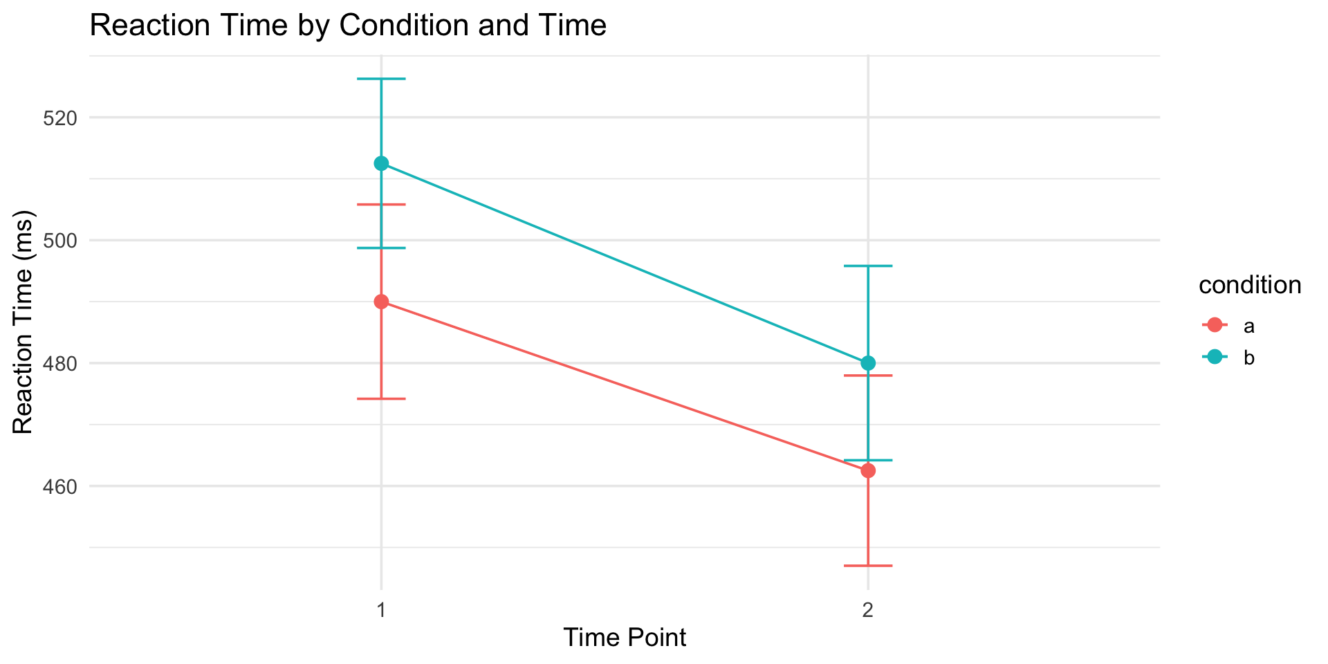
tidy_rm |>
  ggplot(aes(x = time, y = rt, color = condition, group = condition)) +
  stat_summary(fun = mean, geom = "point", size = 3) +
  stat_summary(fun = mean, geom = "line") +
  stat_summary(fun.data = mean_se, geom = "errorbar", width = 0.1) +
  labs(
    title = "Reaction Time by Condition and Time",
    x = "Time Point",
    y = "Reaction Time (ms)"
  ) +
  theme_minimal(base_size = 14)

This is the payoff — show that once the data is tidy, the ggplot code is straightforward. Refer back to the opening slide: “Remember when we couldn’t figure out what to put on the axes? Now we can.” Don’t explain stat_summary() in depth (that’s Session 8); just note that tidy data made this plot possible.

Now we can analyze it!

Example 2: Questionnaire with subscales

# Raw questionnaire data
quest <- tibble(
  pid = 1:3,
  anx_1 = c(3, 2, 4), anx_2 = c(2, 3, 3), anx_3 = c(4, 2, 5),
  dep_1 = c(2, 1, 3), dep_2 = c(3, 2, 4), dep_3 = c(2, 1, 3)
)

quest

# A tibble: 3 × 7
    pid anx_1 anx_2 anx_3 dep_1 dep_2 dep_3
  <int> <dbl> <dbl> <dbl> <dbl> <dbl> <dbl>
1     1     3     2     4     2     3     2
2     2     2     3     2     1     2     1
3     3     4     3     5     3     4     3

Example 2: Questionnaire with subscales

# Tidy and calculate subscales
quest |>
  pivot_longer(
    cols = -pid,
    names_to = c("scale", "item"),
    names_pattern = "(.+)_(.+)",
    values_to = "response"
  ) |>
  group_by(pid, scale) |>
  summarize(subscale_mean = mean(response), .groups = "drop") |>
  pivot_wider(names_from = scale, values_from = subscale_mean)

Example 2: Questionnaire with subscales

# A tibble: 3 × 3
    pid   anx   dep
  <int> <dbl> <dbl>
1     1  3     2.33
2     2  2.33  1.33
3     3  4     3.33

This example shows a pivot_longer() followed by a pivot_wider() — a common real-world pattern. You pivot long to calculate subscale means, then pivot wide again to get one row per participant with separate columns for each subscale. Students often ask: “Why not just do the math in wide format?” You can, but it’s brittle and doesn’t generalize when you have many subscales or items.

Example 3: Multilevel/nested data

# Students nested in classrooms
students <- tibble(
  classroom = rep(c("A", "B"), each = 3),
  student = 1:6,
  pretest = c(70, 75, 72, 68, 71, 69),
  posttest = c(80, 82, 78, 75, 79, 77)
)

students

# A tibble: 6 × 4
  classroom student pretest posttest
  <chr>       <int>   <dbl>    <dbl>
1 A               1      70       80
2 A               2      75       82
3 A               3      72       78
4 B               4      68       75
5 B               5      71       79
6 B               6      69       77

Example 3: Multilevel/nested data

# Tidy for analysis
students |>
  pivot_longer(
    cols = c(pretest, posttest),
    names_to = "time",
    values_to = "score"
  )

# A tibble: 12 × 4
   classroom student time     score
   <chr>       <int> <chr>    <dbl>
 1 A               1 pretest     70
 2 A               1 posttest    80
 3 A               2 pretest     75
 4 A               2 posttest    82
 5 A               3 pretest     72
 6 A               3 posttest    78
 7 B               4 pretest     68
 8 B               4 posttest    75
 9 B               5 pretest     71
10 B               5 posttest    79
11 B               6 pretest     69
12 B               6 posttest    77

pivot_longer() trips everyone up the first time

Pitfall 1: Forgetting what’s a variable

Ask yourself: What are my variables?

• Participant ID? ✓ Variable
• Time point? ✓ Variable (not separate columns!)
• Score? ✓ Variable
• Item number? Depends on your analysis

Students often ask about item number — is it a variable or not? The honest answer is “it depends on your analysis.” If you want per-item analysis, keep it as a variable. If you just want a total score, it’s a grouping artifact. Don’t oversimplify this; acknowledging the ambiguity builds critical thinking about data structure.

Pitfall 2: Over-pivoting

Not everything needs to be long:

# Maybe this is fine as-is?
tibble(
  id = 1:3,
  age = c(25, 32, 28),
  gender = c("M", "F", "F"),
  score = c(85, 92, 88)
)

Age, gender, and score are different variables — keep them as columns.

General tidying strategy

1. Identify the variables (what are you measuring?)
2. Look at your current structure (what’s a row? column?)
3. Determine what operations you need
4. Test with a small subset first
5. Verify you haven’t lost data

Emphasize step 5 — after pivoting, check that you have the expected number of rows. If you started with 3 participants and 4 items, pivot_longer() should give you 12 rows. If it doesn’t, something went wrong. This is a quick sanity check that prevents silent errors. Transition: “Now try the full pipeline yourself.”

Get a head start

Try it yourself

We created wide_rm earlier — a repeated measures dataset:

On your own:

1. Pivot it to long format, extracting condition and time from the column names
2. Calculate mean RT by condition and time
3. Sketch (on paper or in ggplot) what you’d expect the plot to look like

This is very close to what Assignment 3 will ask you to do.

This is individual work, not a pair exercise. Give ~10 minutes if time allows. This uses names_pattern, which is the hardest concept from today. If students are struggling, suggest they start with a simpler pivot (cols = -subject, without names_pattern) to at least get the long format, then try extracting condition and time. Mention that Assignment 3 will involve a very similar task, so this is genuine practice.

Wrapping up

The tidyr toolkit

Function	What it does
pivot_longer()	Wide → Long
pivot_wider()	Long → Wide
separate_*()	Split columns
unite()	Combine columns

The tidy data mantra

1. Each variable is a column
2. Each observation is a row
3. Each value is a cell

When in doubt, ask: “What would make this easiest to plot/analyze?”

Before next class

📖 Read:

• R4DS Ch 7: Data import
• R4DS Ch 20: Spreadsheets

✅ Practice:

• Reshape a dataset you’ve worked with
• Try tidying some messy example data
• Practice pivot_longer() — it’s the most common

Key takeaways

1. Tidy data has a specific structure that works with tidyverse
2. pivot_longer() is your most-used tidying function
3. pivot_wider() is useful for tables and some analyses
4. Think about your variables before reshaping
5. Column names contain information — extract it with names_pattern

The one thing to remember

If your data isn’t tidy, your analysis can’t start. pivot_longer() is the bridge.

Next time: Data Import

End with the reminder about readings for next class (R4DS Ch 7 and Ch 20). If time permits, preview Session 6 briefly: “Next time we’ll learn how to get your own data files into R — CSVs, Excel, SPSS files. You’ll need that skill for every assignment going forward.”