How Many Topics? A Practical Guide to Structural Topic Modeling

I’ve been there: staring at 6,000+ survey responses to an open-ended question, knowing there’s gold in those responses but having no systematic way to find it. Human coding would take months. Reading a random sample might miss rare but critical themes. This is where topic modeling earns its keep.

Topic modeling identifies clusters of words that tend to appear together—latent “topics” in your text data. It’s like factor analysis for language. But here’s the challenge nobody warns you about: there’s no objectively correct number of topics. Unlike clustering algorithms that can optimize for a clear metric, topic modeling requires judgment. And that judgment needs to be informed by both statistics and your research goals.

This post walks through how I approach topic selection and labeling, using real data from a study on COVID-19 vaccine attitudes among parents of young children.

Key Takeaways

There’s no “correct” number of topics. There are useful numbers of topics for your specific purpose.
Use multiple metrics and look for convergence. If exclusivity, coherence, and your own judgment all point to the same solution, you’re probably on solid ground.
Robust topics appear across solutions. If a theme shows up whether you extract 8 or 18 topics, it’s real.
Rare topics aren’t junk topics. Low prevalence might mean low statistical utility, but high importance for understanding edge cases.
Labeling requires reading actual responses. Word clouds are not enough. Look at examples. Argue with a colleague about what to call things. The label is a hypothesis about what the topic means.

The Setup

Our data: 6,516 responses from 3,331 parents answering “How do you feel about the COVID-19 vaccine in terms of its safety and effectiveness, and what are your plans in terms of whether or not to get it?”

The tool: Structural Topic Modeling (STM) in R, which extends standard LDA by allowing you to incorporate covariates. Even if you don’t need covariates, the stm package has excellent tools for model comparison and interpretation.

library(stm)
library(tidytext)
library(tidyverse)
library(ggpubr)
# load data
rapid = read_csv("data/raw_data.csv")

Step 1: Preprocessing (The Boring Part That Matters)

Before modeling, you need to clean the text. This means removing stopwords, numbers, and rare terms. One non-obvious decision: don’t stem your words. Recent work shows stemming doesn’t improve fit and can actually hurt stability—it collapses meaningful distinctions (like “vaccinated” vs. “vaccination”).

temp &lt;- textProcessor(
    documents = rapid$vaccine,
    metadata = rapid,
    lowercase = TRUE,
    removestopwords = TRUE,
    removenumbers = TRUE,
    removepunctuation = TRUE,
    stem = FALSE  # Skip stemming
)

out &lt;- prepDocuments(
    temp$documents,
    temp$vocab,
    temp$meta
)

Step 2: Cast a Wide Net

Here’s where most tutorials go wrong: they tell you to pick one number of topics and run with it. That’s backwards. Instead, estimate a range of models and compare them.

For our vaccine data, the prompt was specific (limiting topic diversity) but we had lots of responses (enabling more topics). I set the range at 3-20:

storage &lt;- searchK(
    out$documents,
    out$vocab,
    K = c(3:20),
    N = 2000,  # Hold-out sample for evaluation
    init.type = "Spectral",
    heldout.seed = 042022
)

This takes a while—about 80 minutes for our data. Run it overnight or on a cluster.

Step 3: The Metrics (And What They Actually Mean)

The searchK output gives you four metrics. Here’s the honest version of what each tells you:

Exclusivity: Do topics have distinctive vocabularies? Higher is better, but increases mechanically with more topics.

Semantic Coherence: Do the top words in each topic actually co-occur in documents? This correlates with human judgment of topic quality—but it’s highest when you have fewer topics. There’s an inherent tradeoff here.

Residuals: How much variance is left unexplained? Lower is better. Values above 1 suggest you need more topics.

Variational Lower Bound: A likelihood measure. Higher is better, though it keeps improving as you add topics.

The key insight: no single metric gives you the answer. You’re looking for inflection points—places where adding one more topic gives you a meaningful improvement or where the next topic starts hurting coherence.

# Plot all metrics
storage$results %>%
  pivot_longer(cols = -K,
               names_to = "metric",
               values_to = "value") %>%
  filter(metric %in% c("lbound", "exclus", "residual", "semcoh")) %>%
  mutate(across(c(K,value), unlist)) %>% 
  ggplot(aes(x = K, y = value, color = metric)) +
  geom_point() +
  geom_line() +
  facet_wrap(~metric, scales = "free") +
  guides(color = "none")

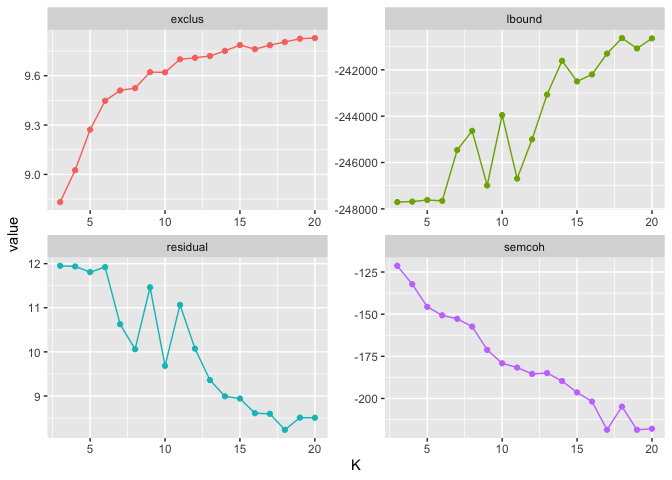
$Metrics for comparing topic modeling\nsolutions.$

In our data, three solutions stood out: 8, 14, and 18 topics. Each represented either a clear improvement over the previous model or preceded a drop in coherence.

Step 4: Fit Your Candidate Models

Now estimate your candidate models in full:

topic_model08 &lt;- stm(
    documents = out$documents,
    vocab = out$vocab,
    K = 8,
    data = out$meta,
    seed = 040122,
    init.type = "Spectral"
)

# Repeat for K = 14 and K = 18

Step 5: Choosing Between Candidates

This is where your research questions matter.

If you need topics as predictors or outcomes: Fewer topics = higher base rates = better statistical power. Rare topics create floor effects.

If you’re exploring for insights or designing future surveys: More topics can surface important distinctions that get collapsed in coarser solutions.

If you’re describing themes for stakeholders: Pick the solution that produces the most interpretable, actionable categories.

Check Topic Prevalence

How often does each topic dominate a response?

# Extract theta (document-topic probabilities)
gamma_08 &lt;- tidy(topic_model08, matrix = "gamma")

# Find dominant topic per document
gamma_08 %>%
  with_groups(document, slice_max, gamma) %>%
  count(topic) %>%
  arrange(desc(n))

## # A tibble: 7 × 2
##   topic     n
##   int int
## 1     6  2034
## 2     1  1619
## 3     3  1248
## 4     7   991
## 5     5   395
## 6     8   141
## 7     4    88

Rare topics (dominating less than 1% of documents) can be valuable for discovering edge cases but problematic for quantitative analysis.

Check Solution Congruence

Which topics appear across all your candidate solutions? These are your most robust themes.

# Extract beta matrices (word-topic probabilities)
beta_08_w &lt;- tidy(topic_model08, matrix = "beta") %>%
  pivot_wider(values_from = beta, names_from = topic)

beta_14_w &lt;- tidy(topic_model14, matrix = "beta") %>%
  pivot_wider(values_from = beta, names_from = topic)

# Correlate across solutions
cor(beta_08_w[,-1], beta_14_w[,-1])

##               1             2             3            4            5
## 1  2.793886e-02  0.0434671930 -0.0127944177  0.007557399  0.549131248
## 2 -5.250151e-04 -0.0028731074  0.1641359131 -0.009513254 -0.003142454
## 3  4.276761e-02  0.0005775644 -0.0207325942  0.601853037  0.052241238
## 4 -5.325039e-03 -0.0026017100  0.1215525469 -0.008026719 -0.003018813
## 5 -9.565136e-04  0.0364205134 -0.0043526821 -0.010482566 -0.003439524
## 6  7.286050e-02  0.0040331021  0.0002033129 -0.011330948 -0.003626186
## 7 -8.319493e-05  0.8176525699  0.0078651678 -0.014767745  0.105715389
## 8  1.218346e-01  0.0986167368  0.2566771685  0.025841438 -0.005438873
##              6            7            8            9          10           11
## 1 -0.006010131  0.008949984 -0.008205705 -0.005073723  0.08502106  0.614189591
## 2 -0.001113922 -0.002818141  0.876105263 -0.002200740 -0.01062583 -0.007538164
## 3  0.001273902  0.170508036 -0.014578379 -0.006711497  0.36329704  0.107947430
## 4  0.748357520 -0.002568847 -0.001885970  0.007322864  0.01432537  0.074573202
## 5 -0.002314192 -0.002921488 -0.002066223  0.410217898 -0.00719231 -0.004446519
## 6 -0.002369077  0.120440743  0.030111250 -0.002295168 -0.01091053 -0.008020140
## 7  0.014731430 -0.003653058  0.009917064 -0.002775218 -0.01107446 -0.008461999
## 8  0.131900205  0.330793407  0.049646161  0.004018404 -0.01759385 -0.011922222
##              12            13            14
## 1 -0.0093451378 -0.0074339247  0.0082637627
## 2  0.0002731391  0.0161673777 -0.0005694858
## 3 -0.0155952699 -0.0147063617 -0.0079572925
## 4  0.3007159746 -0.0028228375 -0.0020555632
## 5  0.4397093343 -0.0003994011  0.6716574995
## 6  0.0792020468  0.8761957963 -0.0021800932
## 7  0.0262934921  0.0524911419 -0.0019696545
## 8 -0.0060075086  0.0231534882 -0.0037929924

Topics that correlate highly across solutions (r > .5) are capturing something real. Topics unique to one solution might be splitting hairs—or might be uncovering something the coarser model missed.

Step 6: Labeling Topics

This is the human judgment part. Use multiple sources of evidence:

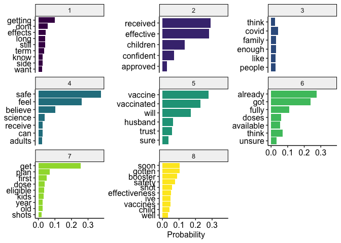
Frequent and Exclusive Words

labelTopics(topic_model08, topics = 4, n = 10)

## Topic 4 Top Words:
##       Highest Prob: safe, feel, believe, science, receive, can, adults, hesitant, felt, positive 
##       FREX: believe, receive, hesitant, felt, needed, house, read, three, anxious, adults 
##       Lift: adults, awesome, follow, hands, house, needed, procedures, process, relative, return 
##       Score: safe, feel, believe, science, adults, receive, hesitant, can, strong, felt

“Frequent” means common in that topic. “Exclusive” means common in that topic and rare elsewhere. Exclusive words are often more diagnostic.

tidy(topic_model08, matrix = "beta") %>% 
    with_groups(topic, top_n, beta, n = 10) %>% 
    filter(beta &gt;= .02) %>% 
    mutate(topic = as.factor(topic)) %>% 
    ggplot(aes(x = reorder(term, beta), y = beta, fill = topic)) +
    geom_bar(stat = "identity") +
    coord_flip() +
    labs(y = "Probability", x = NULL) +
    guides(fill = "none") +
    scale_fill_viridis_d() +
    scale_y_continuous(breaks = seq(0, 1, .1)) +
    facet_wrap(~topic, scales = "free_y") +
    theme_pubr()

Frequent words for 8-topic model.

Key Examples

Read actual responses that score high on each topic:

findThoughts(
    topic_model08,
    texts = out$meta$vaccine,
    topics = c(1),
    thresh = 0.3,  # At least 30% of response assigned to topic
    n = 3
)

## 
##  Topic 1: 
##       Im afraid that they did it too quick and we don't know the effects.  I don't know about getting it.
##      I do not plan on getting it at this time. I am concerned about the side effects or long lasting effects it may have on me.
##      I'm not getting it because I have been advised not to, since it showed chances of blood clots and I'm already on blood thinners because they found a blood clot in my brain while I was still being hospitalized for the stroke.

Setting a threshold prevents loosely-affiliated responses from muddying your interpretation.

Topic Correlations

Which topics cluster together? This can help disambiguate confusing topics:

corr_08 &lt;- topicCorr(topic_model08, cutoff = 0.3)
plot(corr_08)

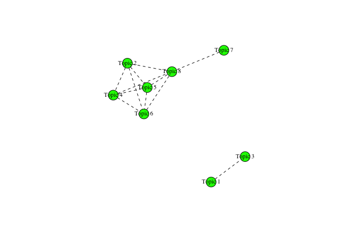
Network plot of topics in 8-topic model.

What We Found

Our 8-topic solution captured broad categories: vaccination status (fully vaccinated, first dose, planning, refusing) and rationale (trust in science, concern about side effects, family considerations).

The 14-topic solution split these further—separating “hesitant but considering” from “firmly opposed,” and distinguishing between concerns about child safety versus personal health.

The 18-topic solution surfaced a rare but important theme: concerns specific to pregnancy and infants. Only 3 documents were dominated by this topic, but for understanding the full landscape of vaccine attitudes? That’s a signal worth having.

Here’s the uncomfortable truth: we used all three solutions in our analysis. Different research questions called for different granularity. The 8-topic model worked for statistical comparisons; the 18-topic model informed our qualitative understanding and helped design follow-up questions.

The full paper with additional code and supplementary materials is available at OSF. All analyses conducted in R using the stm and tidytext packages.